is capable of reliably recovering the signals of interest from much fewer data samples as ..... with corrupted data in DCS scheme and the remaining points can be ...
Derivative Compressive Sampling with Application to Inverse Problems and Imaging by
Mahdi S. Hosseini A thesis presented to the University of Waterloo in fulfilment of the thesis requirement for the degree of Master of Applied Science in Electrical and Computer Engineering
Waterloo, Ontario, Canada, 2010
c Mahdi S. Hosseini 2010
I hereby declare that I am the sole author of this thesis. This is a true copy of the thesis, including any required final revisions, as accepted by my examiners. I understand that my thesis may be made electronically available to the public.
Mahdi S. Hosseini
ii
Abstract In many practical problems in applied sciences, the features of most interest cannot be observed directly, but have to be inferred from other, observable quantities. In particular, many important data acquisition devices provide an access to the measurement of the partial derivatives of a feature of interest rather than sensing its values in a direct way. In this case, the feature has to be recovered through integration which is known to be an ill-posed problem in the presence of noises. Moreover, the problem becomes even less trivial to solve when only a portion of a complete set of partial derivatives is available. In this case, the instability of numerical integration is further aggravated by the loss of information which is necessary to perform the reconstruction in a unique way. As formidable as it may seem, however, the above problem does have a solution in the case when the partial derivatives can be sparsely represented in the range of a linear transform. In this case, the derivatives can be recovered from their incomplete measurements using the theory of compressive sampling (aka compressed sensing), followed by reconstruction of the associated feature/object by means of a suitable integration method. It is known, however, that the overall performance of compressive sampling largely depends on the degree of sparsity of the signal representation, on the one hand, and on the degree of incompleteness of data, on the other hand. Moreover, the general rule is the sparser the signal representation is, the fewer measurements are needed to obtain a useful approximation of the true signal. Thus, one of the most important questions to be addressed in such a case would be of how much incomplete the data is allowed to be for the signal reconstruction to remain useful, and what additional constraints/information could be incorporated into the estimation process to improve the quality of reconstruction in the case of extremely undersampled data. With these questions in mind, the present proposal introduces a way to augment the standard constraints of compressive sampling by additional information related to some natural properties of the signal to be recovered. In particular, in the case when the latter is defined to be the partial derivatives of a multidimensional signal (e.g. image), such additional information can be derived from some standard properties of the gradient operator. Consequently, the resulting scheme of derivative compressive sampling (DCS) iii
is capable of reliably recovering the signals of interest from much fewer data samples as compared to the case of the standard CS. The signal recovery by means of DCS can be used to improve the performance of many important applications which include stereo imaging, interferometry, coherent optical tomography, and many others. In this proposal, we focus mainly on the application of DCS to the problem of phase unwrapping, whose solution is central to all the aforementioned applications. Specifically, it is shown both conceptually and experimentally that the DCS-based phase unwrapping outperforms a number of alternative approaches in terms of estimation accuracy. Finally, the proposal lists a number of research questions which need to be answered in order to attach strong theoretical guarantees to the practical success of DCS.
iv
Acknowledgements I owe my deepest gratitude to my supervisor Professor Ravi Mazumdar for his endless supports. He has made available his support in a number of ways and this thesis would not have been possible without his encouragements and wise advises. I would like to thank Dr. Oleg Michailovich for his great advises and help in the project. I have learned a lot from him. I am heartily thankful to the graduate studies coordinator, Wendy Boles, for her kind and endless help throughout my graduation in the University of Waterloo. I would like to specially thank my friends and colleagues who have helped and inspired me to enjoy of being in Waterloo. My deepest thanks go to Maaj Movahed, Darya Astaraaki, Fariborz Rahimi, Rashin Salehi, Masoud Barakati, Mehri Mehrjoo, Igor Solovy, Elad Shaked, Sudipto Dolui, Amir Goldan and Roham Farzami. Finally, and the most important, I would like to express my deep appreciation to my parents for their endless support, patience, understanding and their true love. As always, I praise God for showing his beauty and power to me by having such wonderful mother and father.
v
to my mother Maryam and father Hossein
& my dear love, Mahta
vi
Contents
Contents
vii
List of Tables
ix
List of Figures
xi
1 Introduction
1
1.1
Problem Statement . . . . . . . . . . . . . . . . . . . . . . . . . . . . . . . .
1
1.1.1
Concept of Sparse Representation . . . . . . . . . . . . . . . . . . . .
3
1.1.2
Augmenting CS with Side Information . . . . . . . . . . . . . . . . .
4
1.2
Applications . . . . . . . . . . . . . . . . . . . . . . . . . . . . . . . . . . . .
4
1.3
Organization of the Proposal . . . . . . . . . . . . . . . . . . . . . . . . . . .
6
2 Literature Review 2.1
8
Phase Unwrapping . . . . . . . . . . . . . . . . . . . . . . . . . . . . . . . .
9
2.1.1
Synthetic Aperture Radar (SAR) Interferometry . . . . . . . . . . . .
9
2.1.2
Principal (Wrapped Phases) . . . . . . . . . . . . . . . . . . . . . . .
11
2.1.3
Residue Theorem and Its Practical Implications . . . . . . . . . . . .
13
2.1.4
Locating Residues in Two-Dimensional Arrays . . . . . . . . . . . . .
15
2.1.5
Quality Maps and Masks . . . . . . . . . . . . . . . . . . . . . . . . .
17
2.1.6
phase Unwrapping in 2D . . . . . . . . . . . . . . . . . . . . . . . . .
21
vii
2.2
2.3
Compressive Sampling . . . . . . . . . . . . . . . . . . . . . . . . . . . . . .
22
2.2.1
Possible Generalization of CS Problem . . . . . . . . . . . . . . . . .
24
2.2.2
Formal Definitions and Underlying Principles . . . . . . . . . . . . .
26
2.2.3
Restricted Isometry Property (RIP) . . . . . . . . . . . . . . . . . . .
29
2.2.4
Kernel Measurements . . . . . . . . . . . . . . . . . . . . . . . . . . .
32
Summary . . . . . . . . . . . . . . . . . . . . . . . . . . . . . . . . . . . . .
34
3 Proposed Method
36
3.1
Derivative Compressive Sampling (DCS) . . . . . . . . . . . . . . . . . . . .
37
3.2
Least-Squares Surface Reconstruction . . . . . . . . . . . . . . . . . . . . . .
39
3.3
Space of Solutions and Its Analysis . . . . . . . . . . . . . . . . . . . . . . .
40
3.3.1
The Problem of Redundant Measurements and Its Solutions . . . . .
43
3.4
Generalization of DCS Problem . . . . . . . . . . . . . . . . . . . . . . . . .
46
3.5
Phase Unwrapping by Means of DCS . . . . . . . . . . . . . . . . . . . . . .
50
3.5.1
Sparse Representation of Image Gradients . . . . . . . . . . . . . . .
50
3.5.2
Data Classification using Quality Maps . . . . . . . . . . . . . . . . .
52
3.5.3
Simulation Results . . . . . . . . . . . . . . . . . . . . . . . . . . . .
52
Summary . . . . . . . . . . . . . . . . . . . . . . . . . . . . . . . . . . . . .
55
3.6
4 Conclusion and Future Plan
59
4.1
Introduction . . . . . . . . . . . . . . . . . . . . . . . . . . . . . . . . . . . .
59
4.2
Proposed Research Plan . . . . . . . . . . . . . . . . . . . . . . . . . . . . .
59
4.3
summary of Contributions and Publications . . . . . . . . . . . . . . . . . .
60
Bibliography
. . . . . . . . . . . . . . . . . . . . . . . . . . . . . . . . . . . . . .
viii
62
List of Tables 3.1
Generalizing the problem of derivative compressive sampling (DCS) compared to conventional compressed sensing (CS) . . . . . . . . . . . . . . . . . . . .
ix
49
List of Figures 1.1
A general structure of DCS - based decoder . . . . . . . . . . . . . . . . . .
2.1
Geometry of SAR interferometry by means of two antennas. S1 and S2 are
3
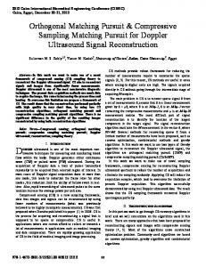
the antennas position. B refers to the baseline of the difference of two sources and Bn refers to the perpendicular baseline. LOS is the line of sight. . . . . 2.2
(a) Original phase; (b) the same phase represented as gray-scale image; (c) Its corresponding wrapped phase. . . . . . . . . . . . . . . . . . . . . . . . .
2.3
10
12
(a) Closed contour evaluated of 2 × 2 pixel neighbourhood of wrapped phase ; (b) A residue maps with its positive and negative pixels indicating the positive and negative residues, respectively. . . . . . . . . . . . . . . . . . . . . . . .
2.4
16
(a) Wrapped phase; (b) Residues of the wrapped phase; (c) Pseudocorrelation map of the wrapped phase; (d) Phase gradient variance of the wrapped phase; (e) Maximum phase y-gradient map; (f) Maximum phase x-gradient map. . .
2.5
19
(a) Mask obtained by thresholding pseudocorrelation quality map; (b) Phase Gradient Variance Mask; (c) Maximum Phase Zy-Gradient Mask; (d) Maximum Phase Zx-Gradient Mask. . . . . . . . . . . . . . . . . . . . . . . . . .
3.1
a) Diagonal spectrum diag (ΛDT D ) of the matrix DT D in Fourier domain; b) Condition number of DT D for different image resolutions . . . . . . . . . . .
3.2
20
44
a) Norm of the projected rows of B to the null-space of AT Γ0 shown in grayvalue; b) Histogram of the norm of the projected rows
x
. . . . . . . . . . . .
46
3.3
(a) Original phase in a ”terrain view”; (b) DCT coefficients of the partial derivative of the phase sorted in descend order; (c) Original phase represented as grayscale image; (d) Its corresponding wrapped phase . . . . . . . . . . .
3.4
51
(a) Phase x-gradient VQM of wrapped phase R; (b) Phase y-gradient VQM of wrapped phase R; (c) x-gradient VQM after applying a threshold of 0.13 ; (d) y-gradient VQM after applying a threshold of 0.13. . . . . . . . . . . . .
3.5
The error surface of phase reconstruction by : (a) DCS; (b) Standard CS; The surface are show as a function of visualized
3.6
. . . . . . . . . . . . . . . . . .
54
(a) Original Terrain; (b) estimate obtained by the standard CS (c) estimate obtained by the proposed DCS method. . . . . . . . . . . . . . . . . . . . . .
3.7
53
56
(a) MSE of phase estimation by DCS method in the presence of introduced noisy measurements varying from 15 db - 35 db. Here, the ratio of random sampling is 38.83% and the method is evaluated and averaged on 20 different noisy scheme for each SNR value; (b) MSE of phase estimation by three different methods: Network-Flow, PUMA, CS and DCS. The total percentage of residual points in measured wrapped phases increases from 1% - 20% . . .
xi
57
Chapter 1 Introduction 1.1
Problem Statement
Reconstruction of signals from random incomplete samples is a task of considerable importance in signal processing, where it belongs to a general class of inverse problems. Factors such as signal corruption due to noises and technical limitations of the acquisition hardware give rise to corrupted or missing data samples, thereby necessitating the developments of methods for signal reconstruction from sub-critically sampled measurements. Compressive sampling (CS) is a framework for finding a solution for such problems by exploiting significant redundancy which may exist in digitally sampled signals. Specifically, compressive sampling relies on two major concepts: sparsity and incoherency, which are properties of the signal of interest and the sensing modality, respectively. Sparsity exemplifies the degree to which the information contained in the signal can be concisely represented in a properly chosen basis Ψ. In other words, the number of non-zero coefficients in basis domain gives a measure of signal compressibility. Incoherency, on the other hand, provides a measure of the degree of similarity between the atoms of sensing (Φ) and representation (Ψ) dictionaries. This notion expands upon the idea of Heisenberg’s uncertainty principle [1–11]. A compressed sensing scheme, which achieves a high degree of reconstruction accuracy, requires the signal of interest to be represented as sparsely as possible in the domain of Ψ. 1
The related representation domain required to be as incoherent as possible with respect to Φ. Unfortunately, finding proper bases Ψ and Φ is not a trivial task, since the definition of Φ is typically constrained by the nature of a data acquisition device at hand. This necessitates the use of specific sensing modality in compressed sensing and since the coherency of the latter should remain low with representation dictionary, finding a proper modal for sparse representation could be a challenge. For instance, numerous applications are known in which one is provided with the measurements of the gradient of a multidimensional signal, rather than of the signal itself [12–18]. Central to such applications is, therefore, the problem of reconstruction of signals from their partial derivatives, subject to some a priori constraints which could be either probabilistic or deterministic in nature. The problem is further complicated when only a subset of the partial derivatives is provided via measurements. In this case the solution involves two concurrent inverse problems and the uncertainty of the scenario becomes more complicated. At the first glance, one might overcome the problem by demonstrating energy minimization methods in order to approximate the corrupted derivatives. Then applying least squares solution to bring approximated derivatives to the spatial domain to represent the estimated signal. In many cases, the signals of interest are the functions of bounded variation whose distributional derivative is a set of locally finite measurement, i.e. f ∈ BV (Ω) where Ω be a open subset of Rn for multi-dimentional space. Therefore, the gradient values can be sparsely represented by choosing proper bases for encoding (e.g., DCT) and the question of whether the partial derivative of an image can be recovered through a compressive sampling (CS) scheme from partial observations must be asked. If so, the estimate of the original signal can be recovered from its recovered gradients by solving a convex optimization problem. The principal contribution of the proposed research is to demonstrate that the performance of such a reconstruction algorithm can be improved via introducing a priori knowledge which exist in the signal of recovery, e.g., cross-derivative equality in the case of partial derivative samples. This proposal introduces a scheme called derivative compressive sampling (DCS), which aims to solve the image recovery inverse problem in two steps. First, image gradients are
2
recovered from an incomplete data set using a modified version of the compressive sampling algorithm. Then, an estimate of the image is recovered from its gradients through solving a least squares problem. Figure 1.1 elaborates on the proposed DCS methodology, to be fully explained in subsequent sections. Among the advantages of such an approach are: • sparse representation of image gradients in a proper basis, e.g., DCT. The sparser is the representation, the fewer data samples are needed to recover the estimate of the signal via compressive sampling. • cross-derivative constraints is incorporated as a priori information to the signal to be recovered. The observed samples along the mentioned side information is an intriguing combination to improve the performance of proposed decoder.
Figure 1.1: A general structure of DCS - based decoder
1.1.1
Concept of Sparse Representation
The image gradient needs to be compressible (sparsely represented) with respect to the properly chosen dictionary Ψ for decomposition. This intriguing challenge of transformation is critical since there is a trade-off between the number of measurements and sparsity level. 3
The most sparse the partial derivatives can be represented, fewer samples will be needed from the signal of interest. This proposal uses a discrete cosine transform (DCT) representation to present our preliminary results as an illustration. However, finding the optimal representation among all possible choices is a future research task to be accomplished.
1.1.2
Augmenting CS with Side Information
The domain to which the compressive sampling framework is applied is that of partial derivatives, which doubles the number of samples used to represent an image. Since the cross-derivative equality constraint must hold, this side information is added as a-priori knowledge of the recovery algorithm in DCS. Imposition of this constraint allows some of the observed samples to be discarded where they already can be incorporated from the crossderivative constraints. This constraint prevents retaining redundant information where the half of the partial derivatives can be interpreted from the related equality.
1.2
Applications
Image interferometry is an important application of remote sensing which allows one to perform earth observation on terrain heights, depth sounding of coastal and ocean depths, weather monitoring, monitoring of glaciers in the Arctic and Antarctic regions, or mine detection [19, 20]. Such sensing makes it possible to remotely collect information from dangerous locations or otherwise inaccessible sources. Aperture synthesis refers to the problem of recovering surfaces of an object using an interferometer. This method combines signals received from individual antennas to provide an image with a resolution declaring the maximum distance between the antennas. This is done by using correlation techniques where the image i(x, y) then is restored by inverse Fourier transform of the measured function of the related coordinates [19]. For instance, interferometric synthetic aperture radar (InSAR) uses two or more antennas to collect the phase difference between antennas and terrain to infer the topography of such areas. In such acquisition systems, phase is measured via modulo-2π so called principle 4
phase value or wrapped phase, i.e., φ = ψ + 2kφ where φ is the true phase value and ψ is the measured quantity. ψ is wrapped between [−π, π] and k ∈ Z is an integer number of wavelength [21]. Phase unwrapping refers to the problem of recovering the true phase φ from wrapped phase ψ. However, the related task is an ill-posed problem if no further information is been provided. This information comes from the Itoh’s condition [22] where it assumes that the absolute value of phase difference between neighbouring pixels is bounded by π. This assumption is no longer been guaranteed if there exist a discontinuity in true phase where it originates from insufficient sampling grids in steep terrain heights (NyquistShannon sampling condition). It can also be originated from noisy measurements where in either cases, phase unwrapping becomes a very difficult problem to solve [21]. Methods which have been introduced to solve the problem of phase unwrapping use a variety of approaches which can be divided into two categories: Path following algorithms [23–25] and minimum Lp -norm solutions [26–33]. Path following algorithms use line integration schemes over wrapped phase image where it relies on the Itoh’s condition to hold along the integration path. This condition along the all possible shortest paths, 2 × 2 neighbouring pixels, is been checked and if it get violated it refers to as inconsistent points so-called residual points. Although many efficient algorithms have been introduced for phase unwrapping in 2-D, most of them nevertheless struggle with the task of interpreting such residual points in their algorithms. These points present ambiguities to the algorithms causing them to fail in successfully unwrapping phase images when the total number of residual points increases in the wrapped images beyond a certain amount. The wrapped version of the difference of wrapped phase is analogous to the derivative of true phase. Since the signal of interest in DCS is the derivative of the signal, this interesting analogy brings the idea whether the problem of phase unwrapping can be fitted to the derivative compressive sampling scheme or not. As mentioned before, residual points brings inconsistency to the phase unwrapping methods, so these points are in direct relationship with corrupted data in DCS scheme and the remaining points can be considered as observed samples. The next challenge is to represent such derivatives sparse in a domain that the dictionary used for sparse representation is highly incoherent with sampling dictionary which is dot-sampling in the case of phase unwrapping. Subsequently, this proposal provides a new 5
solution to the phase unwrapping problem, which compares favourably with other approaches based on the presented preliminary results for terrain height recovery.
1.3
Organization of the Proposal
The remainder of the proposal is organized as follows. Chapter 2 provides a literature review on two major subjects: 2-D phase unwrapping and compressive sampling. Phase unwrapping is discussed in Section 2.1. In this section, the problem of remote sensing and phase measurement is explained. Synthetic aperture radar (SAR) interferometry is stated as an example where the concept of the phase principle values, wrapped phase, is explained. Residual points and its practical implication is elucidated in Subsection 2.1.3. Since the residual points contaminate the measured phase values, Subsection 2.1.4 clarifies how to locate such points in wrapped phases. The quality of measured phase is discussed in Subsection 2.1.5 where it is used as a quality guide map in phase unwrapping process. Many unwrapping algorithms have been introduced in the literature. A short survey on the latter is been exemplified in Subsection 2.1.6. The second portion of the Chapter 2 defines the theory of compressive sampling given in Section 2.2. The origination of the latter is explained and possible generalization of the theory is issued in Subsection 2.2.1. Subsection 2.2.2 provides a formal description of the compressive sampling problem. Stability analysis and recoverability of the CS problem is provided by two types of analysis, one with restricted isometry property (RIP) in Subsection 2.2.3 and the other with distortion of the kernel spaces in Subsection 2.2.4. Chapter 3 presents the formulation of derivative compressive sampling (DCS) as well as the system architecture. Design of the method is explained in Section 3.1. Since the recovered signal via DCS is the image gradient, Section 3.2 applies the least squares solution to recover the image surface from its gradients. Section 3.3 clarifies the space of the solution and necessary number of samples to uniquely recover the signal of interest via DCS. The problem of redundant measurement in DCS is explained in Subsection 3.3.1 and proposes a solution to eliminate non-necessary samples. The DCS is applied on the problem of phase
6
unwrapping and preliminary results are demonstrated in Section 3.5. The following chapter is summarized in Section 3.6. Finally, Chapter 4 outlines the conclusion and the research plan of the following thesis.
7
Chapter 2 Literature Review Since the proposed methodology is derived as a symbiosis of two distinct areas of scientific research - phase unwrapping and compressive sensing - Section 2 provides an overview of existing literature on both fields. First, the problem of phase unwrapping is discussed. Phase unwrapping is a challenging task due to the existence of residual points where they impose ambiguities in unwrapping process. Path following, minimum Lp -norm, bayesian and parametric modelling methods are the main approaches for phase unwrapping algorithms. The second part focuses on the problem of compressed sensing where it expands the main ideas and results. This area has been vastly investigated both in theoretical and applicational aspects. The following chapter is organized as follows. Section 2.1 explains the problem of phase unwrapping. Next, in subsection 2.1.3, the concept of residual points is introduced. These points are known as inconsistent points where subsection 2.1.4 explains the locating methodology in order to incorporate such information to prevent unstability of unwrapping process. The quality of the measured phase at a discrete level is affected by the residual points in wrapped phases. Subsection 2.1.5 gives an analogy to determine such quality by introducing quality maps and subsection 2.1.6 gives a short overview on the existing methodologies for phase unwrapping. As mentioned in Section 1.2, the problem of phase unwrapping can be solved as a specific instance of compressive sampling scheme. The remainder of this chapter gives an overview 8
of the compressive sampling (CS) problem in Section 2.2. The basic intuitions of CS is given in subsection 2.2.2. Based on the analytical improvement of the field, two main categories have been separated in compressive sampling defined in Sections 2.2.3 and 2.2.4 by means of restricted isometry property (RIP) and kernel measurements, respectively. Finally Section 2.3 concludes the chapter.
2.1
Phase Unwrapping
Phase interferometry refers to the technique that infers the direction of the arrival of the signal collected by at least two separated antennas through measuring the difference in phase. This technique is used in many applications to estimate the amplitude differences from the ground. Among such applications are synthetic aperture radar (SAR) imaging [19], magnetic resonance imaging (MRI) [34], fringe pattern analysis [35], tomography and spectroscopy [36]. The phase is collected from the argument of complex functions of transferred signals used to record the data in such applications. The difference in phase magnitude is expressed as an integer number of wavelengths with addition of fraction of one wavelength, so the measured phase lyes between (−π, π] [21].
2.1.1
Synthetic Aperture Radar (SAR) Interferometry
In this subsection, we exemplify the problem of phase unwrapping using the example of synthetic aperture radar (SAR) interferometry as an important application in remote sensing. This imaging technique is of great importance in geophysical monitoring [20]. It provides high resolution images at higher altitudes from the ground regardless of any climate conditions, day or night. It utilizes two or more reflected coherent signals from terrain to elicit relevant phase information through their interference. These signals are sent by an aircraft or satellite platform differ in the sensor flight track, acquisition time or used wavelengths [37]. Figure 2.1 demonstrates the geometry of synthetic aperture radar (SAR) interferometry by means of two antennas S1 and S2 separated by the baseline B. The phase difference between the two SAR images is referred as interferometric phase ∆φ. 9
Figure 2.1: Geometry of SAR interferometry by means of two antennas. S1 and S2 are the antennas position. B refers to the baseline of the difference of two sources and Bn refers to the perpendicular baseline. LOS is the line of sight.
10
For instance, in the case of two coherent signals they can be approximated as � � j4πR1 (x,y) , G1 (x, y) ∼ = A1 (x, y) exp λ � � j4πR2 (x,y) G2 (x, y) ∼ , = A2 (x, y) exp λ
(2.1)
where Ai is the complex terrain reflectivity, Ri is the range from satellite i to the point (x, y) and λ is the microwave’s wavelength [21]. The reflectivity terms are usually highly correlated and can be considered to be equal, i.e., A1 (x, y) = A2 (x, y) = A(x, y). The interferometric phase is related to the difference in the propagation path of the two transmitted signals, so the interfered of the two images can be expressed by conjugate multiplication, � � 4π 2 ∗ G1 (x, y)G2 (x, y) ∼ [R1 (x, y) − R2 (x, y)] , (2.2) = |A(x, y)| exp j λ The phase difference is measured by the argument function operating on the complex quantity in (2.2). This provides wrapped version of the phase, i.e., W (4π/λ) [R1 (x, y) − R2 (x, y)] ∈ (−π, π] . {z } |
(2.3)
∆φ
The wrapping operator W here adds a piecewise constant function to the original interferometric phase ∆φ resulting in W [∆φ] = ∆φ + 2πk, k ∈ Z.
(2.4)
So, in conclusion the wrapped phase lyes between −π ≤ W [φ] ≤ π. The difference in phase originates from the elevation change in the ground where the relation between these two variation builds the topographic mapping, i.e., ∆φ = ∆z
4π Bn λ R sin θ
(2.5)
where θ here is the direction of arrival signal and ∆z is the difference in elevation from the ground [38].
2.1.2
Principal (Wrapped Phases)
As mentioned before, there are different application in phase interferometry that the generated images are wrapped between ±π. Let F (x, y) be an arbitrary continuously differentiable 11
(a)
(b)
(c)
Figure 2.2: (a) Original phase; (b) the same phase represented as gray-scale image; (c) Its corresponding wrapped phase. function defined over a closed subset of the real plane R2 . If F happens to be the phase of a complex-valued function, it can only be measured in its wrapped form, i.e. modulo 2π. Formally, the process of phase wrapping can be represented by its associated operator W : R2 → (−π, π]. In this notation, the wrapped principal phase R is given as R = W [F ]. Specifically, the operator W adds to F a piecewise-constant function K : R2 → {2π k}k∈Z resulting in R = W [F ] = F + K that obeys [39]: −π < W [F (x, y)] ≤ π, ∀(x, y) ∈ R2 .
(2.6)
In complex notation, the gradients of F and R can be defined by applying the following operator ∇=
∂ ∂ i+ j, ∂x ∂y
(2.7)
where i and j denote the unit vectors associated with the x- and y-axis, respectively. Consequently the gradient of R is given by ∇R = ∇W[F ] = ∇F + ∇K.
(2.8)
Finally, applying the wrapping operator W one more time to both sides of (2.8) results in W [∇W[F ]] = W [∇R] = ∇F + ∇K + K 0 . 12
(2.9)
Due the property of operator W to produce the values in interval [−π, π], the term K + K 0 vanishes as long as [21] −π < ∇F ≤ π.
(2.10)
Therefore, as long as the condition (2.10) above holds, the gradient of the original phase F can be unambiguously recovered from the gradient of the corresponding principal phase R according to ∇F = W [∇R] .
(2.11)
Provided (2.11) holds, in 1-D, the original phase can therefore be recovered through integrating the wrapped differences of wrapped phases done by Itoh’s method [22]. The notion can be extended for higher dimensions e.g. 2-D signals (images ) simply considering a path for integration along the phase gradients. In this case, the original phase is estimated by applying an optimization problem, given a measured wrapped phase R, an estimate Fˆ of the original phase F could be obtained as a solution to the following minimization problem
Fˆ = arg min
Z Z
F
k∇F − W{∇R}k2 dx dy,
(2.12)
which amounts to solving a Poisson equation subject to appropriate boundary conditions. Unfortunately, situations are rare in which the condition (2.10) can be a priori guaranteed. In this case, the estimate of ∇F as W[∇R] is contaminated by, so called, residuals, which cause the solution of (2.11) to be of little practical value.
2.1.3
Residue Theorem and Its Practical Implications
As mentioned, the concept of Itoh’s integration method [22] for phase unwrapping can be extended to the case of N dimensions, where by integrating from an initial point r0 any point r can be carried out through a line integral [21], Z F (r) = ∇F · dr + F (r0 ),
(2.13)
∂S
where ∂S is any path in N -dimensional space connecting the points r0 and r and ∇F is the phase gradient field. Assuming ∇F ∈ C 1 is a differentiable vector field defined over 13
a piecewise C 2 bounded oriented surface S ∈ R3 whose boundary ∂S has the inherited orientation, then the line integral in (2.13) is equivalent to the surface integral from Stoke’s theorem Z Z
Z ∇F · dr =
(∇ × (∇F )) · da.
∂S
(2.14)
S
This theorem is also regarded as curved version of Green’s theorem in the plane [40]. An special case of this theory states that if the surface S is a closed surface (∂S = 0) then the path integral of gradient field in (2.13) becomes path independent, i.e., Z Z (∇ × (∇F )) · da = 0.
(2.15)
S
By substituting ∇F = i∂F/∂x + j∂F/∂y and dr = idx + jdy where i and j are coordinate directions in two dimension, the integral in (2.13) along any path ∂S becomes � Z � ∂F ∂F I= dx + dy , ∂x ∂y ∂S
(2.16)
Recalling from the vector calculus, the curl of the gradient vanishes if the cross-derivatives are equal, i.e., � � � � � � �� ∂F ∂F ∂ ∂F ∂ ∂F ∇ × (∇F ) = ∇ × i +j = 0i + 0j + − k = 0, ∂x ∂y ∂y ∂x ∂x ∂y
(2.17)
which happens if and only if ∂ ∂y
�
∂F ∂x
�
∂ = ∂x
�
∂F ∂y
� .
(2.18)
The cross-derivative constraint in (2.18) holds for any differentiable function (gradient field here) ∇F ∈ C 1 where it can be violated in isolated points. In this case, the path integral in (2.16) becomes path dependent. In conclusion, the integral in (2.16) will turn to zero through any closed contour (path) if, and only if, the condition in (2.18) holds, � I � ∂F ∂F dx + dy = 0, (2.19) ∂x ∂y If this condition holds for any closed path, the integration in (2.13) becomes path independent and the wrapped phase can be unwrapped by evaluating the related integral, starting from any initial point. In the case of 2−D phase unwrapping, the condition for path independency (2.18) can be violated if the condition in (2.10) does not hold. The failure of such condition in 14
practical implementation can be motivated by noisy measurements and sub-nyquist sampling problem where it can affect the process of phase unwrapping algorithms [21]. As was mentioned before, the closed loop integration in (2.19) can be non-zero for specific paths if it violates the condition in (2.18). The smallest closed path in two dimensional discrete case can be defined by a 2 × 2 pixel neighbourhood. This small loop can help to locate phase inconsistency in all over the sampled image, where it is called the “residues” by Goldstein et al [23]. The “residue theorem” for two-dimensional phase unwrapping is introduced by the following integration I ∇F · dr = 2π × (sum of enclosed path residue charges),
(2.20)
where it defines that the closed path integral around any residue will equal some integer multiple of 2π radians. The line integral around a balanced residue is equal to zero for any simple path. Thus, two-dimensional phase unwrapping is possible if, and only if, balanced residues lye in all integral paths and the integration do not encircle any unbalanced residues.
2.1.4
Locating Residues in Two-Dimensional Arrays
Locating the residues is a crucial step of phase unwrapping due to the inconsistence information contain in such points. Let Ri,j be the wrapped counterpart of the original phase Fi,j . Recalling Equation (2.11), the wrapped difference of wrapped phase is analogous to the original phase difference, except for the phase residues. Thus, evaluating Equation (2.20) on all phase gradient fields will provide balanced and unbalanced phase residual information for all 2 × 2 pixel closed paths in the image. Lets assume that we have access to the sampled of wrapped phase arrays Ri,j . A small portion of such portion can be modelled as shown in Figure 2.3(a) and the wrapped difference of wrapped phase can be formulated by, ∆yi,j = W {Ri+1,j − Ri,j } , i ∈ {0, . . . , M − 2} , j ∈ {0, . . . , N − 1} ∆yi,j = 0,
(2.21)
otherwise,
and ∆xi,j = W {Ri,j+1 − Ri,j } , i ∈ {0, . . . , M − 1} , j ∈ {0, . . . , N − 2} ∆xi,j = 0,
otherwise, 15
(2.22)
(a)
(b)
Figure 2.3: (a) Closed contour evaluated of 2 × 2 pixel neighbourhood of wrapped phase ; (b) A residue maps with its positive and negative pixels indicating the positive and negative residues, respectively. where reflective boundary conditions are used. x an y superscripts refer to wrapped difference in the j and i indexes, respectively. Integration of the gradient along 2 × 2 pixel closed path, shown in Figure 2.3(a), can be evaluated by summing the phase differences around the closed path. Referring to Figure 2.3(a), ∆1 = ∆yi,j = W {Ri+1,j − Ri,j } ∆2 = ∆xi+1,j = W {Ri+1,j+1 − Ri+1,j } ∆3 = −∆yi,j+1 = W {Ri,j+1 − Ri+1,j+1 }
(2.23)
∆4 = −∆xi,j = W {Ri,j − Ri,j+1 } P ⇒ Residue Charge = 4k=1 ∆k The closed path integral along any 2 × 2 pixel is equal to zero if the cross-derivative condition in (2.18) holds, otherwise there will exist an unbalanced residue of the closed integral with ±2π value. Figure 2.3(b) demonstrates the location of residual point of wrapped phase in Figure 2.2(c). Positive and negative charges are shown by white and black pixels, respectively. Residues mark near origination/termination of end points of disconnected lines in wrapped phase image along which the true phase gradient exceeds ±π. Such disconnected lines are also known as fringe-patterns.
16
2.1.5
Quality Maps and Masks
Residues make the process of phase unwrapping path dependent and the problem turns to be ill-posed. In fact, given a wrapped phase, one can retrieve infinite number of possible corresponding unwrapped images. In many algorithms the performance of unwrapping process depends on how such residues are going to be incorporated in the procedure. For example, in many path-following algorithms, the performance of the methods depends on the path chosen for unwrapping. Goldstain’s brach cut algorithm [23], known as a classical algorithm, is one of fastest methods which connects nearby residues to make them balanced and minimize the length of branch cuts. However, this method is not an optimal solution. In several path following methods [41,42] and weighted Lp -norm solutions [26–29], the measured phase is qualified to guide the unwrapping procedure. This is done by quantifying the quality information generated by residual points. The quality maps are arrays of values which define the quality of given phase data. For each two dimensional wrapped phase we can define a quality map that measures the quality or “goodness” of each pixel in the image [21]. Amongst many maps, the following maps are commonly used in the field of phase unwrapping • Pseudocorrelation is analogous to the correlation map of the complex-valued SAR images, |Qm,n | =
qP P ( cos ψi,j )2 + ( sin ψi,j )2 k2
(2.24)
where the sum are evaluated over a k × k neighbourhood of each pixel (m, n) and ψi,j is the arrayed measured phase. Figure 2.4(c) shows the related Pseudocorrelation map of the wrapped image in Figure 2.4(a). • Phase Derivative Variance is the statistical variance of difference of wrapped phase, r � �2 q P �2 P ∇y ψi,j − ∇y ψ m,n + ∇x ψi,j − ∇x ψ m,n Qm,n = (2.25) k2 where the sum is taken over k × k windows centred at (m, n) pixel in the image. ∇y ψi,j and ∇x ψi,j are the y and x gradients which can be approximated by (2.21) and (2.22), 17
respectively. Finally, ∇y ψ m,n and ∇x ψ m,n are the averages of y and x gradients defined on k × k windows, respectively. This quality map is shown in Figure 2.4(d). • Maximum Phase Gradient defines the largest phase gradient in k × k windows, see Figure 2.4(e) and 2.4(f). � Qym,n = max ∆yi,j � Qxm,n = max ∆xi,j
(2.26)
On phase that remains in constant variation, the phase derivative variance is zero and it differs from pseudocorrelation measure, see Figure 2.4(c) and 2.4(d) for comparison. In addition to the mentioned three quality maps, there is an extra correlation map which is been calculated via tilted baseline, see Figure 2.1 in SAR imaging. This map is the best estimation of the quality of measured phase in SAR imaging since it measures the decorrelated phase caused by SAR layover. The baseline distance B between two antennas S1 and S2 and the tilt of this base line (see Figure 2.1) generates two complex-valued SAR images, ui,j and vi,j , where it generates the correlation map, i.e. ∗ ui,j vi,j , P |ui,j |2 |vi,j |2
P Qm,n = pP
(2.27)
∗ where vi,j is the complex conjugate of vi,j . The sum in (2.27), called “multilook averaging,” is
evaluated over the k×k neighbourhood centred at (m, n) pixels. Among the three introduced quality maps, phase derivative variance highlight the same regions of decorrelated values in correlated map. This quality map is the most reliable one for phase quality measurement when the correlation map data is not available [21]. In order to depict the quality of measured phase, the arrays of the quality map is quantized and variates between [0, 1] increasing from the poor to the best quality. Usually the unwrapping methods require mask for each pixel instead of the quality value in order to depict whether the related pixel is going to be considered in unwrapping procedure or not. So, in practice, the quality map are binarized by means of global thresholding to produce the related mask. Usually this threshold value is extracted by an adaptive method called quality re-mapping [43] or manually by a human factor [42], see Figure (2.5) for the binarized masks. 18
(a)
(b)
(c)
(d)
(e)
(f)
Figure 2.4: (a) Wrapped phase; (b) Residues of the wrapped phase; (c) Pseudocorrelation map of the wrapped phase; (d) Phase gradient variance of the wrapped phase; (e) Maximum phase y-gradient map; (f) Maximum phase x-gradient map.
19
(a)
(b)
(c)
(d)
Figure 2.5: (a) Mask obtained by thresholding pseudocorrelation quality map; (b) Phase Gradient Variance Mask; (c) Maximum Phase Zy-Gradient Mask; (d) Maximum Phase ZxGradient Mask.
20
2.1.6
phase Unwrapping in 2D
An increasing number of research methods have been introduced over the past three decades for two dimensional phase unwrapping. These methods are mainly classified in two parts: path-following algorithms and Lp -norm solutions. Branch cut algorithms by Goldstein et al [23] was introduced in 1988 which is regarded as classical path-following method. The aim of the method was to connect nearby residues with opposite polarities by branch cuts in order to minimize the sum of the cut lengths. The integration path in this method is not allowed to have cross-overs, so the closed loop integral of phase difference in the related path will vanish to zero. The algorithm generates minimum branch cuts and is extremely fast. However, Goldstein algorithm suffers from the noisy measurements since it generates branch-cuts that joins the residues in clumps rather than pairs. Some other branch cut algorithms are addressed in [24] and [25] overcome this problem by restricting the branch-cuts to dipole cuts. The second approach for phase unwrapping is the minimum Lp -norm methods, where these methods try to match local derivatives with measured derivatives “as closely as possible” through minimizing the norm of the error in (2.12). Least squares solution (L2 -norm) first proposed by Fried and Hudgin [26, 27] in 1977 to minimize the sum of squares of gradients between the wrapped phase and reconstructed surface. Fornaro et al [28] improved the method by introducing a weighted mask on the least squares. Ghiglia and Romero [44] developed wighted least square method by combining fast cosine transform and iterative method to unwrap the phase. The L2 -nomr method has also been investigated by Pritt [43] where he used multigrid techniques to solve Gauss-Seidel relaxation schemes. L2 -norm solutions are sensitive to the outliers, so the solution does not pass through the data points exactly. The minimum absolute error occurs where p = 1 where the outliers have lower impact on the solution. The solution to the problems is addressed by Flynn [29] and Costantini [30] where they used discontinuity modelling approaches and network flow for global minimization, respectively. In particular, for the case 0 ≤ p < 1 the discontinuity is preserved as feature of Lp -norm algorithms and enhanced by Chen [31]. Although some of these algorithms are more accurate and stable, but they lack from the computational 21
efficiency and practically heavy to implement. L0 -norm optimized solutions are the most desirable methods in practice. These methods impose a constraint to the solution such that the phase difference of wrapped phase should matches with the unwrapped phase in the sense of minimum L0 -norm. During the process, the weighting coefficients from quality maps are required to mask the phase inconsistencies [21, 45]. Unfortunately, since the L0 -minimization method is non-convex, the search space is non-feasible and the unique minimized solution is not guaranteed. In addition, these methods need combinatorial searching and computationally heavy to implement. Some other unwrapping methods have been introduce where they combine both pathfollowing and minimum Lp -norm methods. Bioucas-Dias and Valado [32] proposed new energy minimization framework (PUMA) in 2007 on phase unwrapping based on graph cuts optimization technique, where the algorithm considers convex pairwise pixel interaction using classical minimum Lp -norm problems for p ≥ 1. Later on, Bioucas-Dias [33] improved the methodology by means of adaptive local de-noising based on local polynomial approximation prior to their phase unwrapping algorithm.
2.2
Compressive Sampling
The idea of sparse signal recovery was first introduced by Donoho [46] in the form of the generalized uncertainty principle. In this initial setup, a band limited signal f (t) ∈ L2 (R) is used for transmission over a channel, in which it “loses” its values on a subset T . Formally, one can define r (t) = (I − PT ) f (t) + n(t),
(2.28)
where I denotes the identity operator (If )(t) = f , n(t) is observation noise, and PT denotes the spatial limiting operator of the form
PT f (t) =
f (t), t ∈ T 0,
22
otherwise
(2.29)
The second operator used in [46] is a band limiting operator defined by Z PΩ f (t) ≡ fˆ(ω)e2πıωt dω,
(2.30)
Ω
where fˆ(ω) denotes the Fourier transform of f (t). The function f and its Fourier transformed fˆ(ω) are mainly concentrated on the measured subsets T and Ω, respectively, such that kf − PT f (t)k2 ≤ �T
(2.31)
ˆ ˆ f − P f (t)
≤ �Ω .
Ω
(2.32)
and 2
By the above assumption, the following theorem is introduced [46]. Theorem 1 Let T and Ω be measurable sets and suppose there is a Fourier transform pair (f, fˆ), with f and fˆ of unit norm, such that f is �T -concentrated on T and fˆ(ω) is �Ω concentrated on Ω. Then the following inequality holds |1 − (�T + �Ω )| ≤ kPΩ PT k ≤
p |Ω| · |T |,
(2.33)
where for the bounded linear operator PT PΩ the norm of the operator is kPT PΩ f k . f ∈L2 (R) kPΩ f k
kPT PΩ k = sup
(2.34)
The operator norm kPT PΩ k measures how a band-limited function (i.e., g ∈ B2 (Ω) implies p PΩ g=g) can be concentrated on T. The inequality kPΩ PT k ≤ |Ω| · |T | implies that there is a limited “energy” concentration on T for band limited signals. For example, if |Ω|·|T | = 0.5 then it implies no band limited function can be located on T with more than 50% of its “energy”. The same theory applies for the finite dimensional signals where the sets T and Ω become index set. The main goal in [46] is to reconstruct the transmitted signal f from the noisy received signal r. The possibility of such a recovery is assured by Theorems 1 above and Theorem 4 in [46] asserting that if |Ω| |T c | < 1, where T c indicates the zero measure set of the function (complement of the set T ), then there exists a linear operator Q and a constant p such that kf − Q[r]k ≤ pknk, 23
(2.35)
� �−1 p where p ≤ 1 − |T c | |Ω| . Specifically, the reconstruction operator Q is given by −1
Q = (I − PT PΩ )
=
∞ X
(PT PΩ )k .
(2.36)
k=0
Moreover, the resulting solution is unique, and it can be approximated by computing a truncated Neumann series for some finite k = N . This interesting result indicates that if a band-limited signal corrupts in the receiver such that |Ω| |T c | < 1 then the signal can be recovered via iterative method introduced by Neumann series. Such condition is analogues to the Heisenberg inequality where the support of the signal in spatial and frequency domains have inverse relation with each other. Over the past two decades, the idea of sparse signal recovery has been generalized and investigated with wavelets analysis. Sparse representation of the signals by means of multiresolutional analysis brought many attentions to the field over the past decade where it originated the concept of compressed sensing to recover signals with fewer sample rates. This concept is in exact opposite definition of Nyquist-Shannon condition, where it indicates that in order to avoid aliasing in signal recovery, the signal should be sampled with twice the frequency exist in the signal. But, compressive sampling propose the idea that if the signal can be represented sparse in a domain then with much fewer sampling rate, the recovery is possible.
2.2.1
Possible Generalization of CS Problem
The theory of “Compressive Sampling (CS)”, also referred as compressed sensing, is a novel pattern of sampling strategy which is against the conventional approach of data acquisition. The theory asserts that one can recover signals of interest with an incomplete measurements compared to traditional method used for signal recovery. This theory has been attracted a lot of attention both in mathematics and application. Generally speaking, this idea refers to recovering n-dimensional signals f approximately from linear measurements hx, φi i where φi ∈ RN may form an orthonormal basis, yi = hf, φi i , i ∈ Ω ⊂ {1, . . . , n} , 24
(2.37)
where m = |Ω| is the cardinality of Ω defines the number of partial indices, usually picked uniformly at random, such that m < n. Let ΦΩ be the n × m matrix whose columns are restricted to φi for which i ∈ Ω. Then, assuming that the signal f can be sparsely represented by a dictionary, for example usually wavelet domains, as f = Ψ c for some coefficient vector c ∈ Rn , the signal can be exactly recovered by solving combinatorial optimization problem (P0 ) minc kck0 s.t. ΦTΩ Ψc = y,
(2.38)
where y ∈ Rm stands the vector of m measurements in (2.11) and kck0 is the number of nonzero components in c. K = # {ci 6= 0, i ∈ {1, . . . , n}}. However, this minimization is a non-convex problem and the searching space is unfeasible, so the unique minimization is not guaranteed. Instead, a more computationally efficient strategy for recovering c from its measurements can be carried out by solving convex L1 -minimization problem (P1 ) minc kck1 =
Pn
k=1
|ck |, s.t. ΦTΩ Ψc = y,
(2.39)
The above problem can be solved by means of linear programming which, among all solutions obeying the measurement constraint ΦTΩ Ψc = y, picks the one that has the sparsest representation in the domain of Ψ as measured by the `1 -norm of c. One can show that, under certain conditions, the problem P0 and P1 are equivalent. For instance , Donoho et al showed in [1] that unique sparse representation cˆ to the solution of P1 is equivalent to P0 if, and only if, k = kˆ ck0 < (1 + 1/M )/2
(2.40)
where M is the mutual coherency of the overcomplete dictionary [Φ, Ψ], M=
max |hφi , ψj i| 1 ≤ i, j ≤ n
(2.41)
i 6= j This result provides a bound on the number of elements of sparse vectors that can be recovered via linear programming LP (P1 ) and allow to construct a matrices [Φ, Ψ] with √ k � n. Recent surveys in compressed sensing [2, 3] provide results in the existence of 25
matrices with k � n/ log (m/n) which is substantially larger than
√
n. Extensive research
has been done in the field to extract bounds for stable recoveries. The sampling rate versus sparsity of the vectors is the main issue to guarantee unique and efficient recoveries.
2.2.2
Formal Definitions and Underlying Principles
The idea of compressive sampling was first formulated by Candes in [4] showing that certain classes of vectors can be recovered from their partial measurements via solving the minimization problem P1. Formally speaking, the necessary and sufficient condition for c to be a unique minimizer of (P1 ) is dependent on the existence of a trigonometric polynomial function P (t). Suppose our sampling is limited to partial information on cˆ such that any solution to (P1 ) should obey, ATΩ c = ATΩ cˆ, Ω ⊂ Zn
(2.42)
where AΩ ∈ Rn×m . Lets define a subset of vectors u ∈ X which has the following features, 1. The support of the vector obeys supp(u) = T = sign(u(t)), t ∈ T 2. There exist a polynomial function P (t) : |P (t)| < 1, t ∈ Tc 3. The polynomial functioned defined be u exist in the kernel of the sensing matrix re� stricted to the complement of the sampled indices Ωc , i.e., P (t) ∈ N ATΩc where supp(.) denotes the support of a function by obtaining the indices where the function is non-zero. The main theorem in [4] can now be stated as follows. Theorem 2 The necessary and sufficient condition for the solution c to be the solution to (P1 ) is that c ∈ X. If this holds, then adding any vector from the kernel of the operator ∀η(t) ∈ ker(AΩ ) will increase the norm, i.e. kc + ηk1 ≥ kck1 . Moreover, if AT Ω is injective, then kc + ηk1 = kck1 which means the minimizer cˆ to (P1 ) is unique and is equal to c. AT Ω here denotes AΩ whose rows are restricted to T . If T ≤ Ω and the matrix AT Ω is of full row rank, then it is injective operator. This theorem states that certain class of vectors 26
which obeying the three conditions above can be the unique minimizer to (P1 ) if the sensing matrix holds injectivity. Analogous results have been driven from uncertainty principles in [46], where it states that if the sparsity level and sampling rate hold |T ||Ω| < n/2, then (P1 ) uniquely recovers the signal of interest. Donoho et al [47] expressed this classical results in more generalized format that c is the unique minimizer to (P1 ) if, and only if, X
X
|c(t) + η(t)| >
t∈Zn
|c(t)| ,
∀η 6= 0, η ∈ ker(AΩ )
(2.43)
t∈Zn
by partition of the left sides of the inequality to T and T c and applying triangle inequality, X
|c(t) + η(t)| =
X
|c(t) + η(t)| +
|η(t)| ≥
t∈T c
t∈T
t∈Zn
X
X
|c(t)| −
t∈T
X
|η(t)| +
t∈T
X
|η(t)| . (2.44)
t∈T c
Hence, the sufficient condition for c to be a unique minimizer of (P1 ) is X
|η(t)|