Derivative compressive sampling with application to ... - CiteSeerX

17th European Signal Processing Conference (EUSIPCO 2009)

Glasgow, Scotland, August 24-28, 2009

DERIVATIVE COMPRESSIVE SAMPLING WITH APPLICATION TO PHASE UNWRAPPING Mahdi S. Hosseini and Oleg V. Michailovich Department of ECE, University of Waterloo 200 University Avenue West, Waterloo, N2L 3G1 Ontario, Canada emails: {smhossei, olegm}@uwaterloo.ca

ABSTRACT Reconstruction of multidimensional signals from the samples of their partial derivatives is known to be an important problem in imaging sciences, with its fields of application including optics, interferometry, computer vision, and remote sensing, just to name a few. Due to the nature of the derivative operator, the above reconstruction problem is generally regarded as ill-posed, which suggests the necessity of using some a priori constraints to render its solution unique and stable. The ill-posed nature of the problem, however, becomes much more conspicuous when the set of data derivatives occurs to be incomplete. In this case, a plausible solution to the problem seems to be provided by the theory of compressive sampling, which looks for solutions that fit the measurements on one hand, and have the sparsest possible representation in a predefined basis, on the other hand. One of the most important questions to be addressed in such a case would be of how much incomplete the data is allowed to be for the reconstruction to remain useful. With this question in mind, the present note proposes a way to augment the standard constraints of compressive sampling by additional constraints related to some natural properties of the partial derivatives. It is shown that the resulting scheme of derivative compressive sampling (DCS) is capable of reliably recovering the signals of interest from much fewer data samples as compared to the standard CS. As an example application, the problem of phase unwrapping is discussed.

cally, the operator W adds to F a piecewise-constant function K : R2 → {2π k}k∈Z resulting in R = W [F] = F + K that obeys [5]: −π < W [F (x, y)] ≤ π, ∀(x, y) ∈ R2 .

In complex notation, the gradients of F and R can be defined as ∂F ∂F i+ j ∂ x1 ∂ x2 ∂K ∂K ∇K = i+ j, ∂ x1 ∂ x2 ∇F =

Numerous applications are known in which one is provided with the measurements of the gradient of a multidimensional signal, rather than of the signal itself. Central to such applications, therefore, appears the problem of reconstruction of signals from their partial derivatives subject to some a priori constraints (which could be either probabilistic or deterministic in nature) [1]. One of such applications, which has been chosen to exemplify the major contribution of this note, is the problem of phase unwrapping. Note that solving this problem is known to be a standard procedure in, e.g., optical and synthethic aperture radar (SAR) interferometry [2], stereo vision [1], blind deconvolution [3, 4], etc. In order to specify the problem of phase unwrapping, let F(x, y) be an arbitrary continuously differentiable function defined over a closed subset of the real plane R2 . If F happens to be the phase of a complex-valued function, it can only be measured in its wrapped form, i.e. modulo 2π. Formally, the process of phase wrapping can be represented by its associated operator W : R2 → (−π, π]. In this notation, the wrapped principal phase R is given as R = W [F]. Specifi-

© EURASIP, 2009

(2)

where i and j denote the unit vectors associated with the xand y-axis, respectively. Consequently, computing the gradient of the wrapped phase R using equations (2) yields ∇R = ∇W[F] = ∇F + ∇K.

(3)

Finally, applying the wrapping operator W one more time to both sides of (3) results in W [∇W[F]] = W [∇R] = ∇F + ∇K + K 0 .

(4)

Due the property of operator W to produce the values in interval [−π, π], the term K + K 0 vanishes as long as [2] −π < ∇F ≤ π.

1. INTRODUCTION

(1)

(5)

Therefore, as long as the condition (5) above holds, the gradient of the original phase F can be unambiguously recovered from the gradient of the corresponding principal phase R according to ∇F = W [∇R] . (6) From the above considerations it follows that, if the condition (5) was known to hold then, given a measured R, an estimate Fˆ of the original phase F could be obtained as a solution to the following optimization problem Fˆ = arg min F

Z Z

k∇F − W{∇R}k2 dx dy,

(7)

which amounts to solving a Poisson equation subject to appropriate boundary conditions. Unfortunately, situations are rare in which the condition (5) can be a priori guaranteed. In this case, the estimate of ∇F as W[∇R] is contaminated by, so called, residuals, which cause the solution of (7) to be of little practical value. In order to overcome the limitations of phase unwrapping inflicted by using the gradients estimated according to (6),

115

a magnitude of different approaches has been hitherto proposed [2]. In the current note, we introduce a different solution to the problem which is based on the concepts of the theory of compressive sampling [5, 6, 7, 8, 9, 10]. In particular, let Γ ⊂ R2 be a finite discrete subset over which the values of F need to be recovered. Let further Γ0 denote a subset of those points in Γ at which the condition (5) is known to hold, and hence at which the gradient ∇F estimated according to (6) can be assumed to be errorless. (Note that the subset Γ0 can be identified based on analysis of the field of residuals as detailed in [2]). Subsequently, we first recover the values of ∇F over the whole Γ from its incomplete measurements over Γ0 , followed by estimating the original phase F using (6). Moreover, in addition to the standard constraints of compressive sampling, we propose to use the constraints stemming from the nature of the gradient as a potential field, viz. ∂ F(x, y) ∂ F(x, y) = . (8) ∂x∂y ∂y∂x We will refer to the problem of reconstruction of F from {∇F(x, y}(x,y)∈Γ0 as the problem of derivative compressive sampling (DCS), and show that using (8) allows considerably reducing the cardinality of Γ0 , while preserving a predefined error rate. The remainder of this paper is organized as follows. Section 2 provides an overview of compressive sampling, and shows how this theory can be used for solution of the problem of phase unwrapping. In Section 3, some necessary technical details are specified. The performance of the method is analyzed in Section 4, while Section 5 finalizes the paper with a discussion and an outline of our future research directions. 2. DERIVATIVE COMPRESSIVE SAMPLING The theory of compressive sampling addresses the problem of perfect reconstruction of signals of interest from their subcritically sampled measurements [5, 6, 7, 8, 9, 10, 11]. In the case when incomplete measurements of the derivatives of the signals are available, the resulting reconstruction problem is refereed to as derivative compressive sampling. 2.1 Basics of Compressive Sampling The idea of compressive sampling was first formulated by D. Donoho [6] in the form of the, so called, generalized uncertainty principle. In this initial setup, a bandlimitted signal f (t) ∈ L2 (R) in used for transmission over a channel, in which it “loses” its values on a subset T . Formally, one can define r (t) = (I − PT ) f (t) + n(t), (9) where I denotes the identity operator, n(t) is observation noise, and PT denotes the spatial limiting operator of the form  f (t), t ∈ T PT f (t) = (10) 0, otherwise The second operator used in [6] is a band-limiting operator defined as given by PΩ f (t) ≡

Z

fˆ(ω)e2πıωt dω,

Ω

where fˆ(ω) denotes the Fourier transform of f (t).

(11)

The main goal of compressive sampling is to reconstruct the transmitted signal f from the noisy recieved signal r. The possibility of such a recovery is assured by Theorems 2 & 4 in [6] asserting that if |Ω| |T c | < 1 (with T c being the complement of T ) there exists a linear operator Q and a constant p such that k f − Q[r]k ≤ pknk, (12)  −1 p where p ≤ 1 − |T c | |Ω| . Specifically, the reconstruction operator Q is given by Q = (I − PT PΩ )−1 =

∞

∑ (PT PΩ )k .

(13)

k=0

Moreover, the resulting solution is unique, and it can be approximated by truncating the Neumann series in (13) at some finite k = N. An addition impetus to the theory of compressive sampling has been given in [7, 8, 9] via introducing the concept of two orthonormal bases Φ and Ψ of Rn , which are used for sampling and signal representation, respectively. Moreover, central to the modern theory of compressive sampling are the notions of • Sparsity, in the sense that signals can be represented by a relatively small number of non-zero coefficients in a properly chosen Ψ, and • Incoherence, which represents the duality between the sampling Φ and representing Ψ domains, where the coherency √ (14) µ(Φ, Ψ) = n max ΦT Ψ remains low. Note that here n is the number of vectors in the basis. In its typical setting, compressive sampling refers to the case when an n-dimensional signals f has to be recovered from its m measurements yk = h f , φk i , k ∈ M ⊂ {1, . . . , n}

(15)

where m = #M and m < n. Let ΦM be the n×m matrix whose columns are formed by those φk for which k ∈ M. Then, assuming that the signal f can be represented as f = Ψ c, for some coefficient vector c ∈ Rn , the reconstruction is carried out via solving n

min kck1 = c

∑ |ck |,

s.t. ΦTM Ψc = y,

(16)

k=1

where y ∈ Rm stands the vector of m measurements in (15). The above problem can be solved by means of linear programming which, among all solutions obeying the measurement constraint ΦTM Ψc = y, picks the one that has the sparsest representation in the domain of Ψ as measured by the `1 -norm of c. Moreover, Theorem 1.2 derived in [10] defines a bound on the number of measurements m m ≥ C µ 2 (Φ, Ψ) S log n

(17)

for which perfect recovery is possible. Note that in (17), C is a constant, while S denotes the number of non-zero elements in ΨT f .

116

2.2 Reconstruction from Partial Derivatives In the case when only partial derivatives of a signal of interest are available, the sampling operator of compressive sampling becomes the kernel of a derivative operator. In particular, in the 2-D case, we are given the measurements of Fx = ∂ F/∂ x and Fy = ∂ F/∂ y. At this point, there are two possibilities to find F. The first would be to define Φ to be a discretized version of the 1st-order derivative operator. This choice, however, could result in relatively large values of the coherency µ(Φ, Ψ) for the case when Ψ is a wavelet orthobasis (which is the choice in the present study). This would, in turn, increase the bound in (17), which could be unacceptable for practical considerations. On the other hand, one can define Φ to be the Dirac comb (i.e., Φ = I). In this case, the partial derivatives can be recovered first, followed by integrating the latter using (7). To proceed with the second of the above-mentioned possibilities, we turn to a discrete setup in which F, Fx and Fy are considered to be n × n matrices. In this case, the maximal possible number of measurements is equal to 2n2 , and hence M ⊂ {1, 2, . . . , 2n2 }. Specifically, we are interested in the case when m = #M < n2 . In 2-D, the partial derivatives Fx and Fy can be approximated according to

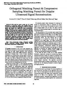
Figure 1: Circular integration paths involving the (i, j) pixel. Using some standard rules of the matrix calculus [12], the above equation can be rewritten as "

#  DT Ψ ⊗ Ψ − Ψ ⊗ DT Ψ vec (cx ) | {z } | {z } = 0 (22) vec (cy ) Bx By {z } | c

The matrix B = [Bx , −By ] is a full (row) rank matrix, whose condition number is approximately equal to 5n/4. In the DCS formulation, this matrix of secondary (crossderivative) constraints is combined with the primary constraints to result in the following optimization problem n2

Fx ' F D

c

Fy ' DT F,

(18)

where D is 2-D difference matrix  1 0 ··· 0  −1 1 ··· 0  0  0 −1 · · · D= .. .. . . ..  . . . .   0 0 ··· 1 0 0 · · · −1

0 0 0 .. . 0 1

       

(19)

  ∇x Ψ cy ΨT = ∇y Ψ cx ΨT . | {z } | {z }

(21)

(23)

k

subject to ⊗ Φ⊗ x Ψ  0 Φ⊗ c Bx

where Gx and Gy are the vectors of measured derivatives. In what follows, the constraints in (20) will be referred to as primary. On the other hand, the cross-derivative (secondary) constraints in (8) can now be expressed as

Fx

k



(Note that the last column of D defines the boundary condition.) For the sake of notational simplicity, let Φ⊗ = Φ ⊗ Φ and Ψ⊗ = Ψ ⊗ Ψ, where ⊗ stands for the Kronecker matrix product. Moreover, since the sampling sets for the xand y-derivatives may be in general different, we denote the ⊗ corresponding sampling matrices by Φ⊗ x and Φy , respectively. Hence, assuming that there exist coefficients cx and cy such that vec(Fx ) = Ψ⊗ vec(cx ) and vec(Fy ) = Ψ⊗ vec(cy ) (with vec denoting the operation of matrix concatenation), the measurement constraints of the DCS problem are defined as ⊗ Φ⊗ x Ψ vec (cx ) = Gx (20) ⊗ vec (c ) = G , Φ⊗ Ψ y y y

Fy

n2

min kck1 = ∑ |cx (k)| + ∑ |cy (k)|,

   0 Gx ⊗ ⊗  Φy Ψ c= Gy −Φ⊗ c By

where Φ⊗ c denotes a sub-sampling operator which removes from the secondary constraints (21) those which are linearly dependent on the primary constraints (20) (see below). Finally, having estimated the partial derivatives Fx and Fy as Ψ⊗ cx and Ψ⊗ cy , respectively, we recover the function (phase) F as a solution to (7). 3. RECOVERING PRIMARY CONSTRAINTS FROM SECONDARY CONSTRAITNS Since the gradient ∇F is a potential field, its integral over any closed path in R2 should be equal to zero, namely I

∇F(s) ds = 0.

(24)

Moreover, in the discrete case, the shortest of such paths connects each 4-pixels neighborhood, as shown in Fig. 1. The shown integration paths result in the following set of equations Fy (i, j) = Fy (i + 1, j) + Fx (i, j) − Fx (i, j + 1) Fy (i, j) = Fy (i − 1, j) + Fx (i − 1, j) − Fx (i − 1, j) Fx (i, j) = Fx (i, j + 1) + Fy (i, j) − Fy (i + 1, j) Fx (i, j) = Fx (i, j − 1) + Fy (i + 1, j − 1) − Fy (i, j − 1) . (25) The constraint equations in (25) can be used to enlarge the set of primary constraints through recovering some of unknown values of Fx and Fy from those of their known neighbors. This procedure can be implemented using Algorithm 1 provided below. q1 : q2 : q1 : q3 :

117

Algorithm 1 Optimal recovery of primary constraint while A pixel can be recovered do for i, j = 1 to n do if all 3 elements in q1 & q2 are knwon then Fy (i, j) = (q1 + q2 ) /2 else if all 3 elements in q1 are knwon then Fy (i, j) = q1 else if all 3 elements in q2 are knwon then Fy (i, j) = q2 end if if all 3 elements in q1 & q3 are knwon then Fx (i, j) = (q1 + q3 ) /2 else if all 3 elements in q1 are knwon then Fx (i, j) = q1 else if all 3 elements in q3 are knwon then Fx (i, j) = q3 end if end for end while

Algorithm 2 Elimination of dependent rows of B for i, j = 1 to n do if Fy (i, j): known AND Fx (i, j): known then if Fy (i + 1, j: known OR Fx (i, j + 1: known then B (i j, :) = [ ] ; end if else if Fy (i, j): known OR Fx (i, j): known then if Fy (i + 1, j): known AND Fx (i, j + 1): known then B (i j, :) = [ ] ; end if else if Fy (i, j): unknown AND Fx (i, j): unknown then if Fy (i + 1, j): known AND Fx (i, j + 1): known then B (i j, :) = [ ] ; end if end if end for

(a)

(b)

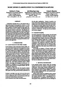
Figure 3: (a) Original phase; (b) Wrapped phase.

Figure 2: Recovering the indices of primary constraint for 256 × 256 test images. Performing Algorithm 1 is a critical step as it maximizes the cardinality of the set of primary constraints, thereby improving the overall probability of recovering the true gradient. Typically, five iterations of the algorithm are sufficient to complete the task. Fig. 2 provides a quantitative characteristics of the algorithm which have been averaged over a number of 256 × 256 test images. Finally, in order to exclude any linear dependency between the primary and secondary constraints, the matrix Φ⊗ c in (23) should be identified. However, in practice, instead of finding the matrix, we simply remove the rows of B which are linearly dependent on the primary constraints. This can be done using Algorithm 2. It should be pointed out that while Algorithm 1 maximizes the number of primary constraints, Algorithm 2 guarantees that the constraint matrix in (23) is of full row rank. After the execution of both algorithms, the problem of recovering the (sparse) representation coefficients c can be solved by linear programming. However, in the 2-D case, such a solution could be rather impractical considering the size of

signals under consideration. To alleviate the computational burden, in the current work, the sparse solutions have been found using the algorithm detailed in [13]. 4. RESULTS We demonstrate the performance of our algorithm using a fringe pattern from the fringe phase data [14]. The original phase and its wrapped version are shown in Figure (3(a)) and (3(b)), respectively. Throughout the experimental study, Ψ was defined to be an orthogonal basis matrix corresponding to the nearly symmetric wavelet of I. Daubechies having six vanishing moments. In our first numerical experiment, we compared the performance of the DCS algorithm with that of the standard CS method. Note that the latter can be obtained from the former by simply discarding the cross-derivative constraints (21). Through analyzing the field of residuals corresponding to the estimated phase gradient (see Fig. 4(b)), 23.76% of the total number of gradient samples were dismissed as unreliable. Fig. (4(a)) shows the unwrapped phase estimated using the DCS algorithm. The mean-squared error (MSE) of the estimation was found to be 0.116%. As a comparison, the same solution was computed using the standard CS, whose MSE was found to be equal to 2.35%. Thus, one can see

118

(a)

(b)

Figure 4: (a) Original phase estimated by the DCS method; (b) Residual points. that augmenting the primary constraints of CS by the crossderivative constraints results in substantial reduction in the level of MSE. In our second experiment, we fixed the MSE of 2.35% as obtained by the standard CS above, and further reduced (via random exclusion) the number of available data points to find the percentage for which the DCS method would result in the same error rate. This percentage was found to be equal to 60%. As a comparison, for the same number of excluded data points, the standard CS resulted in MSE of 8.45%. 5. CONCLUSION The main idea of derivative compressive sampling is to augment the constraints of the standard CS by some additional constraints related to the properties of the gradient as a potential field. In this case, the reconstruction algorithm resolves the ambiguity of “too few samples” not by only looking for a solution of maximal sparseness in the domain of Ψ, but also a solution that complies with the properties of a gradient field. The proposed DCS algorithm is performed in two stages: first, the partial derivatives of a signal of interest are recovered from their sub-critically sampled measurements, followed by integrating the estimated derivatives via solving a Poisson equation. It should be noted, however, that it is possible to get rid of the second stage via defining the sampling system Φ to be a discretized version of the 1st-order derivative operator. In this case, the resulting CS problem should be capable of directly recovering the original signal. Unfortunately, this solution seems to be applicable only for recovering relatively smooth signals. This is because the derivativebased Φ can be incoherent only with bases of smooth (slow varying) functions, thereby ruling out the use of wavelets and the relatives thereof. The current research results leave open a lot of exciting theoretical questions (e.g., as to what other constraints could be incorporated into the problem of CS). Moreover, it is still to be proved what bases could be considered to be optimal for representing the gradients of natural scenes [15]. Computation efficiency of DCS is another issue that should not be overseen when practical applications of DCS are of concern [16].

[1] J. D. Jackson, A. J. Yezzi, and S. Soatto, “Joint priors for variational shape and appearance modeling,” in IEEE Conference on Computer Vision and Pattern Recognition, 2007. CVPR ’07, June 17-22. 2007, pp. 1–7. [2] D. C. Ghiglia, M. D. Pritt, Two-dimensional phase unwrapping: Theory, algorithms, and software. New York: Wiley-Interscience, 1998. [3] O. Michailovich and A. Tannenbaum, “A fast approximation of smooth functions from samples of partial derivatives with application to phase unwrapping,” Signal Processing, Vol. 88, pp. 358–374, 2008. [4] O. Michailovich and D. Adam, “Phase unwrapping for 2-D blind deconvolution of ultrasound images,” IEEE Trans. Med. Imag., vol. 23, No. 1, pp. 7–25, Jan. 2004. [5] A. V. Oppenheim, R. W. Schafer, Discrete time signal processing. London: Prentice Hall, 1989. [6] D. L. Donoho and P. B. Stark, “Uncertainty principles and signal recovery,” SIAM J. Appl. Math, vol. 49, no. 3, pp. 906–931, June 1989. [7] E. Candes, J. Romberg and T. Tao, “Robust uncertainty principles: Exact signal reconstruction from highly incomplete frequency information,” IEEE Trans. Infrom. Theory, vol. 52, no. 2, pp. 489–509, Feb. 2006. [8] E. Candes and T. Tao, “Near optimal signal recovery from random projections: Universal encoding strategies?,” IEEE Trans. Infrom. Theory, vol. 52, no. 12, pp. 4506–5425, Dec. 2006. [9] D. L. Donoho, “Compressed sensing,” IEEE Trans. Infrom. Theory, vol. 52, no. 4, Apr. 2006. [10] E. Candes and J. Romberg, “Sparsity and incoherence in compressive sampling,” Inverse Problems, vol. 23, no. 3, pp. 969–985, 2007. [11] E. Candes and T. Tao, “Decoding by linear programming,” IEEE Trans. Inform. Theory, vol. 51, no. 12, Dec. 2005. [12] J. W. Brewer, “Kronecker products and matrix calculus in system theory,” IEEE Trans. Circuits and Sys. , vol. 25, no. 9, Sep. 1978. [13] E. V. D. Berg and M. P. Frielander, “Probing the pareto frontier for basis pursuit solution,” Technical Report TR-2008-01, Department of CS, Univ. of British Columbia , May. 2008. [14] J. A. Quiroga, D. Crespo and J. A. Gomez-Pedrero R “XtremeFringe : state-of-the-art software for automatic processing of fringe patterns,” Optical Measurment Sys. for Industrial Inspection V, Proc. of SPIE, vol. 6616 66163Y-1, 2007. [15] M. Aharon, M. Elad, and A.M. Bruckstein, “The KSVD: An algorithm for designing of overcomplete dictionaries for sparse representation,” IEEE Trans. On Signal Processing, Vol. 54, no. 11, pp. 4311-4322, Nov. 2006. [16] D. L. Donoho, Y. Tsaig, I. Drori and J. l. Starck, “Sparse solution of underdetermined linear equations by stagewise orthogonal matching pursuit,” Technical Report, Univ. of Stanford, 2006.

REFERENCES

119