Deriving Metric Thresholds from Benchmark Data Tiago L. Alves
Christiaan Ypma
Joost Visser
Software Improvement Group Amsterdam, The Netherlands and University of Minho Braga, Portugal Email:
[email protected]
Software Improvement Group Amsterdam, The Netherlands, and Utrecht University Utrecht, The Netherlands Email:
[email protected]
Software Improvement Group Amsterdam, The Netherlands Email:
[email protected]
Abstract—A wide variety of software metrics have been proposed and a broad range of tools is available to measure them. However, the effective use of software metrics is hindered by the lack of meaningful thresholds. Thresholds have been proposed for a few metrics only, mostly based on expert opinion and a small number of observations. Previously proposed methodologies for systematically deriving metric thresholds have made unjustified assumptions about the statistical properties of source code metrics. As a result, the general applicability of the derived thresholds is jeopardized. We designed a method that determines metric thresholds empirically from measurement data. The measurement data for different software systems are pooled and aggregated after which thresholds are selected that (i) bring out the metric’s variability between systems and (ii) help focus on a reasonable percentage of the source code volume. Our method respects the distributions and scales of source code metrics, and it is resilient against outliers in metric values or system size. We applied our method to a benchmark of 100 object-oriented software systems, both proprietary and open-source, to derive thresholds for metrics included in the SIG maintainability model.
I. I NTRODUCTION Software metrics have been around since the dawn of software engineering. Well-known source code metrics include lines of code, the McCabe complexity metric [1], and the Chidamber-Kemerer suite of object-oriented metrics [2]. Metrics are intended as a control instrument in the software development and maintenance process. For example, metrics have been proposed to identify problematic locations in source code to allow effective allocation of maintenance resources. Tracking metric values over time can be used to assess progress in development or to detect quality erosion during maintenance. Metrics can also be used to compare or rate the quality of software products, and thus form the basis of acceptance criteria or service-level agreements between software producer and client. In spite of the potential benefits of metrics, their effective use has proven elusive. Metrics have been used successfully for quantification, but have generally failed to adequately support subsequent decision-making [3]. To elevate the use of metrics from measurement to decisionmaking, it is essential to define meaningful threshold values. These have been defined for some metrics. For example, McCabe proposed a threshold value of 10 for his complexity
metrics, beyond which a subroutine was deemed unmaintainable and untestable [1]. This threshold was inspired by experience in a particular context and not intended as universally applicable. For most metrics, thresholds are lacking or do not generalize beyond the context of their inception. In this paper, we present a method to derive metric threshold values empirically from the measurement data of a benchmark of software systems. The measurement data for different software systems are first pooled and aggregated. Then thresholds are determined that (i) bring out the metric’s variability between systems and (ii) help focus on a reasonable percentage of the source code volume. We designed our method with several requirements in mind to avoid the problems of thresholds based on expert opinion and of earlier approaches to systematic derivation of thresholds. 1) The method should not be driven by expert opinion but by measurement data from a representative set of systems (data-driven); 2) The method should respect the statistical properties of the metric, such as metric scale and distribution and should be resilient against outliers in metric values and system size (robust); 3) The method should be repeatable, transparent and straightforward to carry out (pragmatic). In our explanation of the method the satisfaction of these requirements is addressed in detail. This paper is structured as follows. Section II presents an overview of earlier attempts to determine thresholds. Section III demonstrates the use of thresholds derived through our method, taking the McCabe complexity metric as example. In fact, this metric is used as a vehicle throughout the paper for explaining and justifying our method. Section IV provides an overview of the method itself. Section V describes our benchmark data. Section VI provides a detailed explanation of key steps of the method. Section VII discusses variants of the method and possible threats. Section VIII provides evidence of the wider applicability of the methodology by generalization to other metrics included in the quality model [4] of the Software Improvement Group (SIG). Finally, Section IX provides conclusions and directions of future work.
In this section we review previous attempts to define metric thresholds. We start by describing works where thresholds are defined by experience. Then, we analyze in detail methodologies that derive thresholds based on data analysis, which are directly related to our methodology. We provide an overview about methodologies that derive thresholds based on error information and from cluster analysis. Finally, we discuss techniques to analyze and summarize metric distributions.
Cantelli’s formula, 1/(1 + k 2 ), should have been used instead. Additionally, this methodology is sensitive to large numbers or outliers. For metrics with high range or high variation, this technique will identify a smaller percentage of observations than its theoretical maximum. In contrast, our methodology was designed to derive thresholds from benchmark data and such is resilient to high variation of data our outliers. Also, while French applies the technique to eight Ada95 and C + + systems, we use 100 Java and C# systems.
A. Thresholds derived from experience
C. Thresholds using error models
Many authors defined metric thresholds according to their experience. For example, for the McCabe metric 10 was defined as the threshold [1], and for the NPATH metric 200 was defined as the threshold [5]. Above these values, methods should be refactored. For the Maintainability Index metric, 65 and 85 are defined as thresholds [6]. Methods whose metric values are higher than 85 are highly-maintainable, between 85 and 65 are moderately maintainable and, smaller than 65 are difficult to maintain. Since these values rely on experience, it is difficult to reproduce or generalize these results. Also, the lack of scientific support can lead to dispute about the values.
Shatnawi et al. [9] investigate the use of Receiver-Operating Characteristic (ROC) method to identify thresholds to predict the existence of bugs in different error categories. They perform an experiment using the Chidamber and Kemerer (CKD) metrics [2] and apply the technique to three releases of Eclipse. Although Shatnawi et al. were able to derive thresholds to predict errors, there are two drawbacks in their results. First, the methodology does not succeed in deriving monotonic thresholds. Second, for different releases of Eclipse, different thresholds were derived. In comparison, our methodology is based only in metric distribution analysis, it guarantees monotonic thresholds and the addition of more systems causes only negligible deviations. Benlarbi et al. [10] investigate the relation of metric thresholds and software failures for a subset of the CDK metrics using linear regression. Two error probability models are compared, one with threshold and one without. For the model with threshold, zero probability of error exists for metric values below the threshold. The authors conclude that there is no empirical evidence supporting the model with threshold as there is no significant difference between the models. El Eman et al. [11] argue that there is no optimal class size based on a study comparing class size and faults. The existence of an optimal size is based on the Goldilocks conjecture which states that the error probability of a class increases for a metric values higher or lower a specific threshold (resembling a U-shape). The studies of Benlarbi et al. [10] and El Eman et al. [11] show that there is no empirical evidence for the threshold model used to predict faults. However, these results are only valid for the specific error prediction model and for the metrics the authors used. Other models can, potentially, give different results. In contrast to using errors to derive thresholds, our methodology derives meaningful thresholds which represent overall volume of code from a benchmark of systems.
II. R ELATED W ORK
B. Thresholds from metric analysis Erni et al. [7] propose the use of mean (µ) and standard deviation (σ) to derive a threshold T from project data. A threshold T is calculated as T = µ + σ or T = µ − σ when high or low values of a metric indicate potential problems, respectively. This methodology is a common statistical technique which, when data is normally distributed, identifies 16% of the observations. However, Erni et al. do not analyze the underlying distribution, and only apply it to one system (albeit using three releases). The problem with this methodology is that the assumption of metrics that are normally distributed is not justified, invalidating the use of this methodology. Consequently, there is no guarantee that 16% of observations will be identified as problematic code. For metrics with high values and high variability, this methodology will identify less than 16% of code, while for metrics with low values or low variability, this methodology will identify more than 16% of code. In contrast, our approach does not make assumption about data normality. Moreover, we apply our methodology to 100 projects, both proprietary and open-source. French [8] also proposes a methodology based on the mean (µ) and standard deviation (σ) but using additionally the Chebyshev’s inequality theorem (whose validity is not restricted to normal distributions). A metric threshold T can be calculated by T = µ + k × σ, where k is the number of standard deviations. According to Chebyshev’s theorem, for any distribution 1/k 2 is the maximal portion of observations outside k standard deviations. As example, to identify a 10% maximum of code, we determine the value of k by resolving 0.1 = 1/k 2 . However, French proposes to divide the Chebyshev formula by two which is only valid for two-tailed symmetric distributions. The assumption of two-tailed symmetric distributions is not justified. For one tailed distributions, the
D. Thresholds using cluster techniques Yoon et al. [12] investigate the use of the K-means Cluster algorithm to identify outliers in the data measurements. Outliers can be identified by observations that appear either in isolated clusters (external outliers), or by observations that appear far away from other observations within the same cluster (internal outliers). However, this algorithm suffers from several shortcomings: it requires an input parameter that affects both the performance and the accuracy of the results, the process of identifying the outliers is manual, after identifying outliers the
algorithm should be executed again, and if new systems are added to the sample the thresholds might change significantly. In contrast, our methodology accuracy is not influenced by input parameters, it is automatic, and stable (the addition of more systems results only in small variation).
TABLE I: Quality profiles: Unit complexity risk: JMule LimeWire FrostWire Vuze
0.4.1 4.13.1 4.17.2 4.0.04
Low
Moderate
High
Very high
70.52% 78.21% 75.10% 51.95%
6.04% 6.73% 7.30% 7.41%
11.82% 9.98% 11.03% 15.32%
11.62% 5.08% 6.57% 25.33%
E. Methodologies for characterizing metric distribution Chidamber and Kemerer [2] use histograms to characterize and analyze data. For each of their 6 metrics, they plotted histograms per programming language to discuss metric distribution and spot outliers in two C++ projects and one Smaltalk project. Spinellis [13] compares metrics of four operating system kernels: Windows, Linux, FreeBSD and OpenSolaris. For each metric, box plots of the four kernels are put side-byside showing the smallest observation, lower quantile, median, mean, higher quantile, highest observation and identify outliers. The box-plots are then analyzed by the author and used to give ranks, + or −, to each kernel. However, as the author states, ranks are given subjectively. Vasa et al. [14] proposes the use of Gini coefficients to summarize a metric distribution across a system. The analysis of the Gini coefficient for 10 class-level metrics using 50 Java and C# system revealed that most of the systems have common values. More, higher Gini values indicate problems and, when analyzing subsequent releases of source code, a difference higher than 0.04 indicates significant changes in the code. Finally, several studies show that different software metrics follow power law distributions [15], [16], [17]. Concast et al. [15] show that for a large Smalltalk system most Chidamber and Kemerer metrics [2] follow power laws. Louridas et al. [16] show that the dependencies of different software artifacts also follow power laws. Wheeldon et al. [17] show that different class relationships follow power laws distributions. All the data analysis studies clearly demonstrate that metrics do not follow normal distributions, invalidating the use of any statistical technique assuming a normal distribution. However all the studies fall short in concluding how to use these distributions, and the coefficients of the distributions, to establish baseline values to judge systems. Moreover, even if such baseline values were established it would not be possible to identify the code responsible for deviations (there is no traceability of results). In contrast, our research is focused on defining thresholds with direct applicability to differentiate software systems, judge quality and pinpoint problems. III. M OTIVATING EXAMPLE Suppose we want to compare the technical quality of four peer-to-peer (P2P) systems. Using the SIG quality model [4] we can arrive to a judgment of technical quality. One of the used metrics is the McCabe metric. Using our method to derive thresholds for the McCabe metric, we obtain 6, 8 and 15 which represent 70%, 80% and 90% of all code in the benchmark. Using these values, quality profiles [4] can be derived by computing the percentage of source lines of code of the methods that fall in each of the following risk categories: ≤ 6 for low risk, ]6, 8] for moderate risk, ]8, 15] for high
Fig. 1: Quality profiles for four P2P systems.
risk, and > 15 for very-high risk. Figure 1 and Table I show the quality profiles of four P2P systems: JMule, LimeWire, FrostWire and Vuze1 . Pinpointing potential problems can be done by looking at the methods that fall in the very-high risk category. Looking at the percentages of the quality profiles we can have an overview about overall complexity. For instance, the Vuze system contains 48% of code in medium or higher risk categories, of which 25% is in the very-high risk category. Finally, quality comparisons can be performed: LimeWire is the least complex of the four systems, with 22% of its code in medium or higher risk categories, followed by FrostWire (25%), then by JMule (30%) and, finally, Vuze (48%). IV. B ENCHMARK - BASED THRESHOLD DERIVATION The methodology proposed in this section was designed according to the following requirements: i) it should respect the statistical properties of the metric, such as scale and distribution; ii) it should be based on data analysis from a representative set of systems (benchmark); iii) it should be repeatable, transparent and straightforward to execute. Figure 2 summarizes the six steps of the methodology. 1. metrics extraction: metrics are extracted from a benchmark of software systems. For each system System, and for each entity Entity belonging to System (e.g. method), we record a metric value, M etric, and weight metric, W eight for that system’s entity. As weight we will consider the source lines of code (LOC) of the entity. As example, for the Vuze system, there is method (entity) called MyTorrentsView.createTabs() with a McCabe metric value of 17 and weight value of 119 LOC. 2. weight ratio calculation: for each entity, we compute the weight percentage within its system, i.e., we divide the entity weight by the sum of all weights of the same system. For each system, the sum of all entities W eightRatio must be 100%. As example, for the MyTorrentsView.createTabs() 1 jmule.org/,
limewire.com/, www.frostwire.com/, www.vuze.com/
TABLE II: Number of systems per technology and license.
1. metrics extraction Legend
System ⇀ (Entity ⇀ Metric × Weight) 2. weight ratio calculation
⇀ map relation (one-to-many relationship)
×
System ⇀ (Entity ⇀ Metric × WeightRatio)
product (pair of columns or elements)
3. entity aggregation
System Represents individual systems (e.g. Vuze)
System ⇀ (Metric ⇀ WeightRatio) 4. system aggregation
Entity Represents a measurable entity (e.g java method) Metric
Metric ⇀ WeightRatio 5. weight ratio aggregation
WeightRatio ⇀ Metric 6. thresholds derivation 70%
Metric
80%
Metric
90%
Represents a metric value (e.g. McCabe of 5) Weight Represents the weight value (e.g. LOC of 10) WeightRatio Represents the weight percentage inside of the system (e.g. entity LOC divided by system LOC)
Metric
Fig. 2: Summary of the methodology steps.
method entity, we divide 119 by 329, 765 (total LOC for Vuze) which represents 0.036% of the overall Vuze system. 3. entity aggregation: we aggregate the weights of all entities per metric value, which is equivalent to computing a weighted histogram (the sum of all bins must be 100%). Hence, for each system we have a histogram describing the distribution of weight per metric value. As example, all entities with a McCabe value of 17 represent 1.458% of the overall LOC of the Vuze system. 4. system aggregation: we normalize the weights for the number of systems and then aggregate the weight for all systems. Normalization ensures that the sum of all bins remains 100%, and then the aggregation is just a sum of the weight ratio per metric value. Hence, we have a histogram describing a weighted metric distribution. As example, a McCabe value of 17 corresponds to 0.658% of all code. 5. weight ratio aggregation: we order the metric values in ascending way and take the maximal metric value that represents 1%, 2%, ..., 100% of the weight. This is equivalent to computing a density function, in which the x-axis represents the weight ratio (0-100%), and the y-axis the metric scale. As example, according to the benchmark used for this paper, for 60% of the overall code the maximal McCabe value is 2. 6. thresholds derivaton: thresholds are derived by choosing the percentage of the overall code we want to represent. For instance, to represent 90% of the overall code for the McCabe metric, the derived threshold is 14. This threshold is meaningful, since not only it means that it represents 90% of the code of a benchmark of systems, but it also can be used to identify 10% of the worst code. As a final example, the SIG uses thresholds derived by choosing 70%, 80% and 90% of the overall code, which derive
Technology Java C#
License
n
LOC
Proprietary OSS Proprietary OSS Total
60 22 17 1 100
8,435K 2,756K 794K 10K 11,996K
TABLE III: Number of systems per functionality. Functionality type Catalogue or register of things or events Customer billing or relationship management Document management Electronic data interchange Financial transaction processing and accounting Geographic or spatial information systems Graphics and publishing tools or system Embedded software for machine control Job, case, incident or project management Logistic or supply planning and control Management or performance reporting Mathematical modeling (finance or engineering) Online analysis and reporting Operating systems or software utility Software development tool Stock control and order processing Trading Workflow support and management Other Total
n 8 5 5 3 12 2 2 3 6 8 2 1 6 14 3 1 1 10 8 100
thresholds 6, 8 and 14, respectively. This allows to identify code to be fixed in long-term, medium-term and short-term, respectively. Furthermore, these percentiles are used in quality profiles to characterize code according to four categories: low risk (between 0 − 70%), moderate risk (70 − 80%), high risk (80 − 90%) and very-high risk (> 90%). We present an analysis of these steps in Section VI. V. B ENCHMARKING DATA We applied our methodology for deriving thresholds to a fairly representative set of available software systems. This set includes 100 systems in modern object-oriented technologies (Java and C#), both proprietary from SIG customers and opensource, developed by different organizations, from a broad range of domains. All the 100 systems were used (additional systems considered as outliers were removed from the initial set of systems). The system sizes range from over 3K LOC to near 800K LOC, with a total of near 12 million LOC. Table II specifies the number of systems per technology (Java or C#) and license type (proprietary or open-source). Table III characterizes the used software systems according to their functionality using the taxonomy defined by ISBSG in [18]. For each system we derived metrics at two levels. At method level, LOC (unit size), McCabe (unit complexity) and number of parameters (unit interfacing) were derived. At file level, fan-in (module inward coupling) and number of methods (module interface size) were derived. The choice of these metrics was motivated by their use in the quality model used
(a) Histogram
(b) Quantiles
Fig. 3: McCabe distribution for Vuze system represented with a histogram and a quantile plot. ¨ Informationstechnik (TUViT) ¨ by SIG and TUV for software certification [19] which is an extension of the quality model proposed by Heitlager et al. [4]. All metrics were calculated with the SIG Software Analysis Toolkit (SAT) version 3.2.0. Outlier systems were removed by first inspecting the distribution of metrics. Systems whose distributions are radically different from other system’s distributions were considered outliers. The identified systems were only removed after the outlier suspicion was validated by experts with knowledge about the systems. As rule-of-thumb, we found useful to apply the outlier-detection technique used for box-plots on the 50% quantile: all systems whose value is higher than the upper quantile plus 1.5 IQR is considered a possible outlier. VI. A NALYSIS OF THE METHODOLOGY STEPS The methodology introduced in Section IV makes two major decisions: weighting by size, and using relative size as weight. In this section, based on data analysis we provide thorough explanation about these decisions that are the fundamental part of our methodology. Also, we investigate the representativeness of the derived thresholds. Section VI-A, introduces the statistical analysis and plots used throughout the paper. Section VI-B, provides a detailed explanation about the effect of weighting by size. Section VI-C shows the importance of the use of relative size when aggregating measurements from different systems. Finally, in Section VI-D we provide evidence of the representativeness of the derived thresholds by applying the thresholds to the benchmark data and checking the results. We discuss variants and threats in Section VII. A. Background A common technique to visualize a distribution is to plot a histogram. Figure 3a depicts the distribution of the McCabe values for the Vuze system. The x-axis represents the McCabe values and the y-axis represents the number of methods that have such a McCabe value (frequency). Figure 3a allows us to observe that more than 30.000 methods have a McCabe value ≤ 10 (the frequency of the first bin is 30.000). Histograms, however, have several shortcomings. The choice of the bins affects the shape of the histogram possibly
(a) Non-weighted
(b) Weighted
Fig. 4: McCabe distribution for the Vuze system (nonweighted and weighted by LOC) annotated with the x and y values for the first three changes of the metric.
causing misinterpretation of data. Also, it is difficult to compare the distributions of two systems when they have different sizes since the y-axis can have significantly different values. Finally, histograms are not very good to represent the bins with lower frequency. To overcome these problems, an alternative way to examine a distribution of values is to plot its Cumulative Density Function (CDF) or the CDF inverse, the Quantile function. Figure 3b depicts the distribution of the McCabe values for the Vuze system using a Quantile plot. The x-axis represents the percentage of observations (percentage of methods) and the y-axis represents the McCabe values. The use of the quantile function is justifiable, because we want to determine thresholds (the dependent variable, in this case the McCabe values) as a function of the percentage of observations (independent variable). Also, by using the percentage of observations instead of the frequency, the scale becomes independent of size of the system making it possible to compare different distributions. In Figure 3b we can observe that 96% of methods have a McCabe value ≤ 10. Despite that histograms and quantile plots represent the same information, the quantile plot allows better visualization of the full metric distribution. Therefore, in this paper all distributions will be depicted with quantile plots. All the statistical analysis and charts were done with R [20]. B. Weighting by size Figure 4a depicts the McCabe distribution for the Vuze system already presented in Figure 3b in which we annotated the quantiles for the first three changes of the McCabe value. We can observe that up to the 66% quantile the McCabe value is 1, i.e. 66% of all methods have a metric value of 1. Up to the 77% quantile, the McCabe values are smaller than or equal to 2 (77−66 = 11% of the methods have a metric value of 2), and up to the 84% quantile have a metric value smaller than or equal to 3. Only 16% of methods have a McCabe value higher than 3. Hence, Figure 4a shows that the metric variation is concentrated in just a small percentage of the overall methods. Instead of considering every method equally (every method has a weight of 1), we will use the method’s LOC as its weight.
(a) All quantiles
(b) All quantiles (cropped)
(a) Full distribution
(b) Cropped distribution
Fig. 6: Summarized McCabe distribution. The line in black represents the summarized McCabe distribution. Each gray line depicts the McCabe distribution of a single system.
(c) All weighted quantiles
(d) All weighted quantiles (cropped)
Fig. 5: Non-weighted and weighted McCabe distributions for 100 projects of the benchmark. (a) Distribution mean differences
Figure 4b depicts the weighted distribution of the McCabe values for the Vuze system. Hence, instead of having the percentage of methods in the x-axis, we will have now the percentage of LOC. Comparing Figure 4a to Figure 4b, we can observe that in the weighted distribution the variation of the McCabe values starts much earlier. The first three changes for the McCabe values are at 18%, 28% and 36% quantiles. In sum, for the Vuze system, both weighted and nonweighted plots show that large McCabe values are concentrated in just a small percentage of code. However, while in the non-weighted distribution the variation of McCabe values happen in the tail of the distribution (66% quantile), for the weighted distribution the variation starts much earlier, at the 18% quantile. Figure 5 depicts the non-weighted and weighted distributions of the McCabe metric for 100 projects. Each line represents an individual system. Figures 5a and 5c depict the full McCabe distribution and Figures 5b and 5d depict a cropped version of the previous, restricted to quantiles higher than or to 70% and to a maximal McCabe value of 100. When comparing Figure 4 to Figure 5 we observe that, as seen for the Vuze system, weighting by LOC emphasizes the metric variability. Hence, weighting by LOC not only emphasizes the difference between methods in a single system, but also make the differences between systems more evident. A discussion about the correlation of the LOC metric with other metrics and the impact of it on our methodology is presented in Section VII-A.
(b) Quality profiles variability
Fig. 7: McCabe variability
C. Using relative size To derive thresholds we need to summarize the metric, i.e., we need to aggregate the measurements from all systems. To summarize the metric, we first perform a weight normalization step. For each method we compute the percentage of LOC that method represents in the system, i.e. we divide the method’s LOC by the total LOC of the system it belongs to. This represents Step 2 of our methodology, presented in Figure 2. Then, we just use all measurements together. Conceptually, to summarize the McCabe metric, we have taken all curves of density functions for all systems and combined them into a single curve. Performing weight normalization ensures that every system is represented equally in the benchmark, limiting the influence of bigger systems over small systems in the overall result. Figure 6 represents the density functions of the summarized McCabe metric (plotted in black) and the McCabe metric for all individual systems (plotted in gray), also shown in Figure 5d. As expected, the summarized density function respects the shape of individual system’s density function. A discussion of alternatives to summarize a metric distribution are presented in Section VII-B. D. Choosing percentile thresholds We have observed in Figures 5 and 6 that systems differentiate the most in the last quantiles. In this section we present
evidence that it is justifiable to choose thresholds in the tail of the distribution and that the derived thresholds are meaningful. Figure 7a quantifies the variability of the McCabe distribution between systems. The full line depicts the McCabe distribution (also shown in Figure 6) and the dashed lines depict the MAD above the distribution and below the distribution. The MAD is a measure of variability defined as the mean of the absolute differences between each value and a central point. From Figure 7a we can observe that both the MAD above and below the curve increase rapidly towards the last quantiles (it has a similar shape as the metric distribution itself). In sum, from Figure 7a, we can observe that the variability between systems is concentrated in the tail of the distribution. It is important to take this variability into account when choosing a quantile for deriving a threshold. Choosing a quantile for which there is very low variability (e.g. 20%) will result in a threshold which will not allow to distinguish quality between systems. Choosing a quantile for which there is too much variability (e.g. 99%) might fail to identify code in many systems. Hence, to derive thresholds it is justifiable to choose quantiles from the tail of the distribution. As part of our methodology we proposed the use of the 70%, 80% and 90% quantiles to derive thresholds. For the McCabe metric, using our benchmark, these quantiles yield to thresholds 6, 8 and 14, respectively. Now we are interested to investigate if the thresholds are indeed representative of those percentages of code. For that, we computed quality profiles for each system in our benchmark. For low risk, we considered the lines of code for methods with McCabe between 1 − 6, for moderate risk 7 − 8, for high risk 9 − 14, and for very-high risk > 14. This means, that for low risk we expect to identify around 70% of the code, and for each of the other risk categories 10%. Figure 7b depicts a box plot for all systems per risk category. The x-axis represents the four risk categories, and the y-axis represents the percentage of volume (lines of code) of each system per risk category. The size of the box is the interquartile range (IQR) and is a measure of variability. The vertical lines indicate the lowest/maximum value within 1.5 IQR. The crosses in the charts represent systems whose risk category is higher than 1.5 IQR. In the low risk category, we observe large variability which is explained because it is considering a large percentage of code. For the other categories, from moderate to very-high risk, we can observe that variability increases. This increase of variability was also expected, since we have observed that the variability of the metric is higher for the last quantiles of the metric. We can observe that there are only a few crosses per risk category, which indicates that most of the systems are represented by the box plot. Finally, for all risk categories, looking to the line in the middle of the box, the median of all observations, we observe that indeed the median is according to our expectations. For low risk category, the median is near 70%, while for other categories the median is near 10% which indicates that the derived thresholds are representative of the chosen percentiles. Summarizing, the box plot shows that the derived thresholds
allow to observe differences between systems in all risk categories. Also, as expected, we can observe that around 70% of the code is identified in the low risk category and around 10% is identified for the moderate, high and very-high risk categories since the boxes are centered around the expected percentages for each category. VII. VARIANTS AND THREATS In this section we present a more elaborated discussion and alternatives taken into account regarding the two decisions in our methodology: weighting with size, and using relative size. Additionally, we discus other issues regarding removal of outliers and issues affecting metric computation. Section VII-A we discuss the reasoning behind using LOC to weight the metric and possible risks due to correlation between metrics. Section VII-B discusses the need of aggregating measurements using relative weight, and discusses other possible alternatives to achieve similar results. Section VII-C explains how to identify outliers and the criteria to remove them. Finally, Section VII-D explain the impact of using different tools or configurations when deriving metrics. A. Weight by size A fundamental part of our methodology is the combination of two metrics, more precisely, a metric for which thresholds are going to be derived with a size metrics such as LOC. In some contexts, particular attention should be paid when combining two metrics. For instance, when designing a software quality model it is desirable that each metric measures a unique attribute of the software. When two metrics are correlated it is often the case that they are measuring the same attribute. In this case only one should be used. We acknowledge such correlation between McCabe and LOC. The Spearman correlation value between McCabe and LOC for our data set (100 systems) is 0.779 with very-high confidence (pvalue < 0.01). In our methodology, the combination of metrics has a different purpose. We use LOC as a measure of size and use it to have a better representation of the part of the system we are characterizing. Instead of assuming every unit (e.g. method) of the same size, we take its size in the system measured in LOC. When doing this, we observed that we emphasized the variation of the metric allowing a more clear distinction between software systems. Hence, the correlation between LOC and other metrics poses no problem. When referring to the LOC metric we could mean either logical or physical lines of code. In any case, since these metrics are highly correlated similar results are expected. Other LOC metrics could also be considered, however the study of such alternatives is deferred to future work. B. Use of relative weight In Section VI-C we advocate the use of relative weight to aggregate measurements from all systems. The reasoning is that, since all the systems have similar distributions, the overall result should represent all systems equally. If we consider all
(a) Effect of large systems in aggre- (b) Mean, Median as alternatives to gation. Relative Weight.
(a) McCabe distribution with an out- (b) McCabe characterization with lier. and without an outlier.
Fig. 8: Effect of using relative weight in the presence of large systems and comparison with alternatives.
Fig. 9: Example of outliers and outlier effect on the McCabe characterization.
measurements together without applying any aggregation technique the large systems (systems with a bigger LOC) would influence the overall result. Figure 8a compares the influence of size between simply aggregating all measurements together (black dashed line) and using relative weight (black full line) using as example the Vuze and JMule McCabe distributions (depicted in gray). Vuze has about 330 thousand LOC, while JMule has about 40 thousand LOC. We can observe that the dashed line is very close to the Vuze system meaning that the Vuze system has a stronger influence in the overall result. In comparison, using the relative weight results in a distribution in the middle of the Vuze and JMule distributions as depicted in the full line. Hence, it is justifiable to use the relative weight since it allows us to be size independent and it takes into account all measurements in equal proportion. In alternative to the use of relative weight we could consider taking the mean/median quantile for all systems. Since the mean/median are measures of central tendency, we could compute the distributions for every system (as shown in gray in Figure 6) and then, take the mean/median value of all distributions per quantile. Figure 8b compares the relative weight to mean quantile and median quantile. As we can observe the result distributions shape is similar although thresholds for the 70%, 80% and 90% quantiles would be different. There are also problems with the mean/median. The mean is a good measure of central tendency if the underneath distribution is normal. We applied Shapiro-Wilk test [21] for normality for all quantiles and verified that the distribution is not normal. Additionally, the mean is sensitive to extreme values, and would favor higher values when aggregating measurements. The median, on the other hand, relies on the order of the distributions to take a central value just taking into account the value of the central point, ignoring information. Additionally, for the last quantiles, the median relies on few data points, i.e., very few methods fall in the last quantiles, meaning that the distribution in the last quantiles will be sensitive to the addition of new data points. Finally, by using the mean/median the metric maximal value will not correspond to the maximal observable value, hiding information about the metric distribution. For our benchmark, the maximal McCabe
value is 911. However, from Figure 8b, for the mean and median, we can observe that values of the metric for the 100% quantile (maximal value of the metric) are much lower. C. Outliers In statistics, it is common practice to check for the existence of outliers. An outlier is an observation whose value is distant relative to a set of observations. According to Mason et al. [21], outliers are relevant because they can obfuscate the phenomena being studied or may contain interesting information that is not contained in other observations. There are several strategies to deal with outliers: remove observations, or use outlier-resistant techniques. In our analysis, we compared the distribution of metrics between systems. Figure 9a depicts the distribution of the McCabe metric for our data set of 100 systems (in gray) plus one outlier system (in black). We can observe that the outlier system has a metric distribution radically different from the other systems. Figure 9b depicts the effect of the presence of the outlier when summarizing the McCabe metric. The full line represents the curve that summarizes the McCabe distribution for 100 systems, previously shown in Figure 6, and the dashed line represents the result of the 100 systems plus the outlier. From Figure 9b, we can observe that the presence of the outlier has limited influence in the overall result, meaning that our methodology has resilience against outliers. D. Impact of the tools/scoping The computation of metric values and metric thresholds can be affected by the measurement tool and by scoping. Different tools implement different variations of the same metrics. Taking as example the McCabe metric, some tools implement the Extended McCabe metric, while other might implement the Strict McCabe metric and also call it McCabe. As the values from these metrics can be different, the computed thresholds can also be different. To overcome this problem, the same tool should be used both to derive thresholds and to analyze systems using the derived thresholds. The configuration of the tool with respect to which files to include or exclude in the analysis (scoping) also influences the
(a) Metric distribution
(b) Box plot per risk category
Fig. 10: Unit size (method size in LOC)
(a) Metric distribution
(b) Box plot per risk category
(a) Metric distribution
(b) Box plot per risk category
Fig. 12: Module Inward Coupling (file fan-in)
(a) Metric distribution
(b) Box plot per risk category
Fig. 11: Unit interfacing (number of parameters)
Fig. 13: Module Interface Size (number of methods per file)
computed thresholds. For instance, the existence of unit test code, which contains very little complexity, will result in lower threshold values. On the other hand, the existence of generated code, which normally have very high complexity, will result in higher threshold values. Hence, it is extremely important to know which data is used for calibration. As previously stated, for deriving thresholds we removed both generated code and test code from our analysis.
results are again similar. Except for the unit interfacing metric, the low risk category is centered around 70% of the code and all others are centered around 10%. For the unit interfacing metric, since the variability is relative small until the 80% quantile we decided to use 80%, 90% and 95% quantiles to derive thresholds. For this metric, the low risk category is a round 80%, the moderate risk is near 10% and the other two around 5%. Hence, from the box plots we can observe that the thresholds are indeed recognizing code around the defined quantiles.
VIII. T HRESHOLDS FOR SIG’ S Q UALITY M ODEL METRICS Throughout the paper, the McCabe metric was used as case study. To investigate the applicability of our methodology to other metrics, we repeated the analysis for the SIG quality model metrics. We found that our methodology can be successfully applied to derive thresholds for all these metrics. Figures 10, 11, 12, and 13 depict the distribution and the box plot per risk category for unit size (method size in LOC), unit interfacing (number of parameters per method), module inward coupling (file fan-in), and module interface size (number of methods per file), respectively. From the distribution plots, we can observe, as for McCabe, that for all metrics both the highest values and the variability between systems is concentrated in the last quantiles. Table IV summarizes the quantiles used and the derived thresholds for all the metrics from the SIG quality model. As for the McCabe metric, we derived quality profiles for each metric using our benchmark in order to verify that the thresholds are representative of the chosen quantiles. The
IX. C ONCLUSION A. Contributions We proposed a novel methodology for deriving software metric thresholds and a calibration of previously introduced metrics. Our methodology improves over others by fulfilling three fundamental requirements: i) it respects the statistical properties of the metric, such as metric scale and distribution; ii) it is based on data analysis from a representative set of systems (benchmark); iii) it is repeatable, transparent and straightforward to carry out. These requirements were achieved by aggregating measurements from different systems using relative size weighting. Our methodology was applied to a large set of systems and thresholds were derived by choosing specific percentages of overall code of the benchmark. B. Discussion Using a benchmark of 100 object-oriented systems (C# and Java), both proprietary and open-source, we explained
TABLE IV: Metric thresholds and used quantiles for the SIG quality model metrics. Metric / Quantiles Unit complexity Unit size Module inward coupling Module interface size Metric / Quantiles Unit interfacing
70% 6 30 10 29 80% 2
80% 8 44 22 42 90% 3
90% 14 74 56 73 95% 4
in detail our methodology for the McCabe metric. We have shown that the distribution of the metric is preserved and that the methodology is resilient to the influence of large systems or outliers. Thresholds were derived using 70%, 80% and 90% quantiles and checked against the benchmark to show that thresholds indeed represent these quantiles. The analysis of these results was replicated with success using four other metrics from the SIG quality model. Variants in our methodology for deriving threshold were analyzed as well as threats to our methodology. Our methodology has proven capable to derive thresholds for all the metrics of the SIG quality model. For unit interfacing the 80%, 90% and 95% was used since the metric variability only increases much later than for other metrics. Thresholds for all other metrics were derived using 70%, 80% and 90%. For all metrics, our methodology showed that the derived thresholds are representative of the chosen quantiles. C. Industrial applications The thresholds derived with our methodology have been successfully used in practice by SIG for software analysis [4], benchmarking [22] and certification [23]. Thresholds based on expert opinion have been replaced by thresholds derived with our methodology which have been used with success. Our methodology has also been applied for other metrics. Luijten et al. [24] found empirical evidence that systems with higher technical quality have higher issue solving efficiency. The thresholds used for classifying issue efficiency were derived using the methodology described in this paper. D. Future work Several avenues of future work are foreseen. Empirical studies to validate software metrics with external qualities, using metric thresholds, such as the one from Luijten et al. [24] are foreseen. Techniques to characterize curves based on a fixed number of points, such as proposed by Schwetlick et al. [25] could be used to choose the quantiles to better characterize the metric distribution. Finally, it would be interesting to apply our methodology to suites of metrics proposed by others, e.g. to the CDK metrics [2], or to metrics for other types of software artifacts, e.g. databases or XML schemas. ACKNOWLEDGMENTS Thanks to Harro Stokman and Joost Schalken for inspiring discussions, to Jos´e Pedro Correia by the support of extracting the metrics, and to several other colleagues of the SIG for
providing comments to earlier versions of this work. The first author is supported by the Fundac¸a˜ o para a Ciˆencia e a Tecnologia, grant SFRH/BD/30215/2006. R EFERENCES [1] T. J. McCabe, “A complexity measure,” Software Engineering, IEEE Transactions on, vol. SE-2, no. 4, pp. 308–320, Dec. 1976. [2] S. R. Chidamber and C. F. Kemerer, “A metrics suite for object oriented design,” IEEE Trans. Softw. Eng., vol. 20, no. 6, pp. 476–493, 1994. [3] N. E. Fenton and M. Neil, “Software metrics: roadmap,” in ICSE Future of SE Track, 2000, pp. 357–370. [4] I. Heitlager, T. Kuipers, and J. Visser, “A practical model for measuring maintainability,” International Conference on the Quality of Information and Communications Technology (QUATIC’07), pp. 30–39, 2007. [5] B. A. Nejmeh, “NPATH: a measure of execution path complexity and its applications,” Commun. ACM, vol. 31, no. 2, pp. 188–200, 1988. [6] D. Coleman, B. Lowther, and P. Oman, “The application of software maintainability models in industrial software systems,” J. Syst. Softw., vol. 29, no. 1, pp. 3–16, 1995. [7] K. Erni and C. Lewerentz, “Applying design-metrics to object-oriented frameworks,” in METRICS ’96: Proceedings of the 3rd International Symposium on Software Metrics. Washington, DC, USA: IEEE Computer Society, 1996, p. 64. [8] V. A. French, “Establishing software metric thresholds,” International Workshop on Software Measurement (IWSM’99), 1999. [9] R. Shatnawi, W. Li, J. Swain, and T. Newman, “Finding software metrics threshold values using ROC curves,” Journal of Software Maintenance and Evolution: Research and Practice, 2009. [10] S. Benlarbi, K. E. Emam, N. Goel, and S. Rai, “Thresholds for objectoriented measures,” in ISSRE ’00: Proc. of the 11th International Symposium on Software Reliability Engineering. IEEE, 2000, p. 24. [11] K. El Emam, S. Benlarbi, N. Goel, W. Melo, H. Lounis, and S. N. Rai, “The optimal class size for object-oriented software,” IEEE Trans. Softw. Eng., vol. 28, no. 5, pp. 494–509, 2002. [12] K.-A. Yoon, O.-S. Kwon, and D.-H. Bae, “An approach to outlier detection of software measurement data using the K-means clustering method,” in ESEM’07. IEEE Computer Society, 2007, pp. 443–445. [13] D. Spinellis, “A tale of four kernels,” in ICSE’08. New York, NY, USA: ACM, 2008, pp. 381–390. [14] R. Vasa, M. Lumpe, P. Branch, and O. Nierstrasz, “Comparative analysis of evolving software systems using the gini coefficient,” in ICSM’09. IEEE Computer Society, 2009, pp. 179–188. [15] G. Concas, M. Marchesi, S. Pinna, and N. Serra, “Power-laws in a large object-oriented software system,” IEEE Trans. Softw. Eng., vol. 33, no. 10, pp. 687–708, 2007. [16] P. Louridas, D. Spinellis, and V. Vlachos, “Power laws in software,” TOSEM’08, vol. 18, no. 1, Sep 2008. [Online]. Available: http: //portal.acm.org/citation.cfm?id=1391984.1391986 [17] R. Wheeldon and S. Counsell, “Power law distributions in class relationships,” SCAM’03, vol. 0, p. 45, 2003. [18] C. Lokan, “The Benchmark Release 10 - project planning edition,” International Software Benchmarcking Standards Groups Ltd., Tech. Rep., February 2008. ¨ [19] Software Improvement Group (SIG) and TUV Informationstechnik ¨ ¨ GmbH (TUViT), “SIG/TUViT evaluation criteria – Trusted Product Maintainability, version 1.0,” 2009. [20] R Development Core Team, R: A Language and Environment for Statistical Computing, R Foundation for Statistical Computing, Vienna, Austria, 2009, ISBN 3-900051-07-0. [21] R. L. Mason, R. F. Gunst, and J. L. Hess, Statistical Design and Analysis of Experiments, 2nd ed. Wiley, 2003. [22] J. P. Correia and J. Visser, “Benchmarking technical quality of software products,” in WCRE ’08: Proceedings of the 2008 15th Working Conference on Reverse Engineering. Washington, DC, USA: IEEE Computer Society, 2008, pp. 297–300. [23] ——, “Certification of technical quality of software products,” in Proc. of the Int’l Workshop on Foundations and Techniques for Open Source Software Certification, 2008, pp. 35–51. [24] B. Luijten and J. Visser, “Faster defect resolution with higher technical quality of software,” in SQM ’10: Proc. of the 4th International Workshop on Software Quality and Maintainability, 2010. [25] H. Schwetlick and T. Sch¨utze, “Least squares approximation by splines with free knots,” 1995.