Design and Implementation of a Low Complexity VLSI ... - CiteSeerX

Journal of VLSI Signal Processing Systems 24, 43–57 (2000) c 2000 Kluwer Academic Publishers, Boston. Manufactured in The Netherlands. °

Design and Implementation of a Low Complexity VLSI Turbo-Code Decoder Architecture for Low Energy Mobile Wireless Communications SANGJIN HONG AND WAYNE E. STARK Wireless Communications Research Laboratory, Department of Electrical Engineering and Computer Science, 1301 Beal Avenue, University of Michigan, Ann Arbor MI 48109-2122 Received April 14, 1999; Revised July 15, 1999

Abstract. Channel coding is commonly incorporated to obtain sufficient reception quality in wireless mobile communications transceiver to counter channel degradation due to intersymbol interference, multipath dispersion, and thermal noise induced by electronic circuit devices. For low energy mobile wireless communications, it is highly desirable to incorporate a decoder which has a very low power consumption while achieving a high coding gain. In this paper, a sub-optimal low-complexity multi-stage pipeline decoder architecture for a powerful channel coding technique known as “turbo-code” is presented. The presented architecture avoids complex operations such as exponent and logarithmic computations. The turbo-code decoding algorithm is reformulated for an efficient VLSI implementation. Furthermore, the communication channel statistic estimation process has been completely eliminated. The architecture has been designed and implemented with the 0.6 µm CMOS standard cell technology using Epoch computer aided design tool. The performance and the circuit complexity of the turbo-code decoder are evaluated and compared with the other types of well-known decoders. The power consumption of the lowcomplexity turbo-code decoder is comparable to that of the conventional convolutional-code decoder. However, the low-complexity turbo-code decoder has a significant coding gain over the conventional convolutional-code decoders and it is well suited for very low power applications.

1.

Introduction

In mobile wireless communications, high performance and low power operation of the portable terminals are desirable. With emergence of personal communication services, portable terminals such as mobile telephones and notebook computers are expected to be used more frequently and for longer times, and hence power consumption will become an important consideration. Thus, the fact of having a battery with limited lifetime is relevant at many levels, and achieving a better power efficiency is a challenge for the designers of mobile wireless communication systems. In typical wireless communication systems, the power amplifier at the transmitter RF front-end dissipates a significant portion of overall transceiver power. The amount of dissipated power by the power amplifier is greatly influenced by communicating channel

environment such as multipath fading, intersymbol interference, thermal noise induced by the electronic RF circuit devices, and other time varying channel degradation. In addition, a distance between transmitter and receiver greatly influences the transmission power. Thus, reduction in the transmission power is the primary concern for low-energy communication system design with maintaining sufficient reception quality for reliable data communication. One way to reduce the transmission power is to incorporate powerful forward error correction (FEC) codes to increase coding gain at the receiver which translates in less transmission power [1–3]. However, Shannon showed that the development of error correction techniques with increasing coding gain has a limit, arising from the channel capacity [4]. Since that work, many different types of codes have been designed and their decoding algorithms are physically realized. They mainly

44

Hong and Stark

differ in decoding performance and their hardware complexity. Traditionally, the Viterbi algorithm has been widely accepted as a choice for decoder for wireless communications because it is an optimum decoding algorithm for the convolutional-code. It performs a maximum likelihood (ML) detection of the state sequence of a finite-state discrete-time Markov process observed in memoryless noise [5]. It can also be interpreted as searching for the minimum-distance path in a trellis by dynamic programming [6], where the measure of distance is the log-likelihood of the corresponding statetransition based on the symbols received over noisy channel. Moreover, many power efficient implementations have been proposed [7–9]. Thus, it is of great interest for a low power communication system which has a low hardware complexity, possibly comparable to the convolutional decoder but has higher coding gain. Recently, a novel class of binary parallel concatenated recursive systematic convolutional-codes termed Turbo-Codes was introduced [10, 11]. These codes have an amazing error correcting capability and are very attractive for applications to digital mobile radio to combat channel fading. The main draw back is that the decoding operation is very complex for practical VLSI realization [12]. The decoding is based on MAP (maximum a posteriori probability) decoders and requires many complex operations such as exponent and logarithmic calculus as well as extensive channel statistic estimation process. Furthermore, a very long duration of data interleaving and deinterleaving processes is needed for achieving the performance as advertised. As the demand for battery powered portable wireless communication applications increases, a minimization of power consumption becomes an increasingly critical concern for integrated circuit design. One of the primary objectives in the design of low-energy communication system is power reduction. Power consumption is the guiding principle for both algorithm development and system trade-off evaluation. The tremendous savings in power consumption can be attained through both algorithm reformulation and architectural innovation specifically targeted for energy conservation. The architecture presented in this paper incorporates a low-complexity design for the low-energy mobile wireless communication applications. Although some VLSI implementations have already been obtained for particular turbo-code decoders [13–15], most of these decoders require MAP decoding algorithm

which has a significant complexity over the conventional convolutional-code decoders. This work is aimed to reduce a considerable amount of algorithmic and circuit complexity for a low power architectural solution that is comparable to the complexity of the convolutional-code decoders. Design efforts are made at the algorithmic level for reducing power dissipation. The proper reformulation of algorithm results in an architecture that is efficiently realizable. And the decoding iteration process is implemented as a multi-stage pipeline. The resulting decoder architecture consumes the power that is comparable to the conventional convolutional decoder but with a significant coding gain. The decoder can be incorporated into the very low power applications, and possibly replacing the convolutional decoder without losing any considerable power efficiency. We first review turbo-codes. The encoding scheme and the decoding algorithm are briefly described. Then, the low-complexity sub-optimal decoding algorithm is reformulated where many complex operations have been eliminated. A simple mechanism for channel estimation is discussed. Based on the reduced complexity decoding algorithm, the VLSI multistage pipeline turbo-code decoder architecture design is presented [16]. A further circuit complexity is minimized by appropriately choosing the finite quantization wordlength. Finally, the performance and the circuit complexity of the decoder are evaluated. The lowcomplexity turbo-code decoder is compared with various well-known decoders in terms of their relative complexity. 2.

Turbo-Code Reviewed

In this section, a turbo-code encoding scheme and its decoder structure are briefly described. The nature of the turbo-code decoding algorithm is iterative and the decoder structure that corresponds to a single iteration is considered in the discussion. Throughout the discussion, additive white Gaussian channel is assumed. 2.1.

Turbo-Code Encoding

Turbo-codes are the parallel concatenation of at least two recursive systematic convolutional (RSC) encoders with interleaving [10–17] as shown in Fig. 1. The code rate of the turbo-code encoder is 1/3, mapping N data bits to 3N code bits. The recursive encoders

Low-Complexity VLSI Turbo-Code Decoder Architecture

Figure 1.

A RSC turbo-code encoding scheme. Figure 2.

are necessary to attain the exceptional performance provided by the turbo-codes. We assume that the constituent codes are identical. The input to each RSC encoder is the same information bit sequence dk but in different order due to the presence of an interleaver. The interleaver takes bit sequence dk and rearrange them in a pseudo-random fashion prior to encoding by the second RSC encoder. For an input bit sequence {dk }, the RSC turbo-code encoder output is {Dk } = {dk }, {C1,k }, and {C2,k }. This allows that low-weight codewords produced by a single RSC encoder are transformed in high-weight codewords for the turbo-code encoder, so achieving high coding gains [11]. The encoding is frame oriented using a finite number of N bits per frame and the trellis of the first RSC encoder is terminated to maintain boundary condition of the trellis path. 2.2.

45

Turbo-Code Decoder Structure

A complete turbo-code decoder structure corresponding to one iteration of the algorithm includes two component decoders, implementing a-posteriori probability, and interleavers/deinterleavers, which scramble the processed data according to the interleaving laws used in the encoder. Other blocks are required such as RAM memories for storing data through the iterations. These block can be interconnected in the decoder in many topologies [18], depending on the encoder structure. In Fig. 2 shows a turbo-code decoder structure for the RSC turbo-code encoder shown in Fig. 1. At each time instant k, there are three different types of soft inputs to the component decoder: the disturbed systematic information x = (x1 , . . . , x N ), the redundant information y 1 = (y1,1 , . . . , y1,N ), and the apriori information (extrinsic information) about the information bit L 2 = (L 2,1 , . . . , L 2,N ). The soft output generated by the component decoder at time instant k contains a weighted version of xk , a weighted version of L 2,k , and a newly generated extrinsic information

RSC turbo-code decoder structure.

L 1,k . L 1,k is a combination of the influences of all soft inputs except for the weighted versions of xk and L 2,k . The newly generated extrinsic information L 1,k is used as the a-priori information of the second component decoder which operates in a similar way to the first component decoder. The transmitted symbols Dk , C1,k , C2,k correspond to the received symbols xk , y1,k , y2,k , respectively. The bi-phase shift keying (BPSK) modulation scheme is assumed in this paper. The log-likelihood ratios (LLRs) are perfect soft information in the case of binary codes [19]. With the abbreviation Rk = (xk , y1,k , L 2,k ),the LLR 3k of bit dk is given by [10] 3k

µ

¶ Pr{dk = 0 | Rk } = ln Pr{dk = 1 | Rk } ! ÃP M m=1 Pr{dk = 0, Sk = m, Rk } = ln P M m=1 Pr{dk = 1, Sk = m, Rk } ! ÃP M P M P1 j 0 0 0 m=1 m 0 =1 j=0 γk (Rk , m , m)αk−1 (m )βk (m) = ln P M P M P1 j 1 0 0 m=1 m 0 =1 j=0 γk (Rk , m , m)αk−1 (m )βk (m)

(1)

where Sk , which can assume values m between 1 and M (the size of trellis), is the state of the first RSC encoder at time k. The forward recursion can be expressed as αki (m) =

1 M X X m 0 =1 j=0

γki (Rk , m 0 , m)αk−1 (m 0 ) j

(2)

and the backward recursion is given by βk (m) =

1 M X X m 0 =1 j=0

γk+1 (Rk+1 , m 0 , m)βk+1 (m 0 ). (3) j

46

Hong and Stark

The branch transition metric is given by

− ln

γki (Rk , m 0 , m) = exp(1/σ 2 · xk · (1 − 2 · i)) · exp(1/σ · y1,k · (1 − 2c1,k )) ¢ ¡ · exp 1/σ L2 · L 2,k · (1 − 2 · i)

×

2

(4)

= ln

M M X X m=1

£

0 (m 0 ) αk−1

M X

βk (m)

¤

1 + αk−1 (m 0 ) M X

× ln

M X

βk (m)

M X

¤ £ 0 1 (m 0 ) + αk−1 (m 0 ) × αk−1 M X

A potential difficulty in physically realizing the turbocode decoding algorithm, which overshadows the benefit of large coding gain, is that it requires many complex arithmetic operations. In addition, in order to achieve high coding gain, the decoding process requires a large number of iterations. These two factor greatly influence the feasibility of low-power physical realization of the decoding algorithm. One solution is to derive a sub-optimal decoder architecture that eliminates high speed processing and reduces the number of complex arithmetic operators (i.e., multiplications and logarithmic operations). However, the decoding performance degradation due to these transformations should minimal.

By using the inequalities

3.1.

max{ζ1 , ζ2 , . . . , ζ M } ≤ ln

Component Decoder Complexity Reduction

− ln

γk1 (Rk , m 0 , m)

× αk−1 (m 0 )βk (m) j

+

βk (m)αk1 (m)

(8)

m=1

Since βk (m) and αki (m) are exponential functions, lets define α˜ ki (m) = ln αk (m) and β˜ki (m) = ln βk (m). Then 3k = ln

M X

¡ ¢ exp β˜k (m) + α˜ k0 (m)

m=1

− ln

M X

¡ ¢ exp β˜k (m) + α˜ k1 (m)

(9)

m=1

M X

exp{ζm }

m=1

≤ ln M + max{ζ1 , ζ2 , . . . , ζ M }.

(10)

˜ k can be expressed as the approximated LLR 3 ª © ˜ k ≈ max α˜ k0 (m) + β˜k (m) 3 m ª © − max α˜ k1 (m) + β˜k (m) m

(11)

α˜ ki (m) (5)

= ln

1 αk−1 (m 0 )

¤

M 1 X X j=0

γk0 (Rk , m 0 , m)βk (m)

m=1 m 0 =1 £ 0 (m 0 ) × αk−1

M X

(7)

The new forward recursion formula α˜ ki (m) is

m=1 m 0 =1 j=0

= ln

βk (m)αk0 (m) − ln

m=1

j γk0 (Rk , m 0 , m)αk−1 (m 0 )βk (m)

M X 1 M X X

M M X X

= ln

m

For a practical low complexity VLSI implementation, it is highly desirable that the decoder should avoid complex arithmetic operations and variance estimation procedure. To compute the extrinsic information, the original formulas must be simplified considerably. The LLR can be approximated as follows

m=1 m 0 =1 j=0

γk1 (Rk , m 0 , m)

m 0 =1

m=1

Low-Complexity RSC Turbo-Code Decoder Integration

3k = ln

γk0 (Rk , m 0 , m)

¤ £ 0 1 (m 0 ) + αk−1 (m 0 ) × αk−1

where σ 2 is the variance of the white Gaussian noise, σ L2 is the variance of L 2,k , and i takes either 0 or 1.

M X 1 M X X

(6)

m 0 =1

m=1

3.

γk1 (Rk , m 0 , m)βk (m)

m 0 =1

= ln

m 0 =1

M X m 0 =1

γki (Rk , m 0 , m)αk−1 (m 0 ) j

¡ 0 ¢ 1 γki (Rk , m 0 , m) αk−1 (m 0 ) + αk−1 (m 0 )

(12)

(13)


≈ ln

M X

0 γki (Rk , m 0 , m)αk−1 (m 0 )

m 0 =1

+ ln

M X

¢ ¡ 1 γki Rk , m 0 , m)αk−1 (m 0 )

(14)

m 0 =1

≈ ln

M X

¡ ¢ 0 exp γ˜ki (Rk , m 0 , m) + α˜ k−1 (m)

m 0 =1

+ ln

M X

¡ ¢ 1 exp γ˜ki (Rk , m 0 , m) + α˜ k−1 (m)

(15)

m 0 =1

ª © 0 1 (m 0 ) α˜ k−1 (m 0 ), α˜ k−1 ≈ γ˜ki (Rk , m 0 , m) + max 0 m

(16)

where γ˜ki (m) = ln γk (m). Throughout this paper, the approximate equality will be removed and the new forward recursion formula can be rewritten as © 0 ª 1 α˜ ki (m) = γ˜ki (Rk , m 0 , m) + max α˜ k−1 (m 0 ), α˜ k−1 (m 0 ) (17) Similarly, the new backward recursion formula can be written as ) ( 1 (Rk+1 , m, m 0 ) + β˜k+1 (m 0 ) γ˜k+1 ˜ βk (m) = max 0 (18) γ˜k+1 (Rk+1 , m, m 0 ) + β˜k+1 (m 0 ) where m 0 is a possible source state to m in the trellis. The branch metrics are defined as γ˜ki (Rk , m 0 , m)

= xk · (1 − 2 · i) + y1,k · (1 − 2 · c1,k ) + L 2,k · (1 − 2 · i)/Q p

(19)

assuming that the channel condition remains constant during the duration of the data block (so that σ 2 is fixed assuming the additive white Gaussian channel with no fading within the duration of a data block). The weighting factor Q is defined as Q p = σ L2, p /σ 2

for p = 0, 1, 2, . . . , P − 1

(20)

where p represents iteration index and P represents the maximum number of iterations allowed. Thus σ L2, p indicates the value of σ L2 at the pth iteration. 3.2.

Choice of Weighting Factor Q

Assuming a constant σ 2 , the weighting factor Q p is proportional to the value of σ L2, p . The value of σ L2, p serves as reliability of the extrinsic information L at pth iteration. The smaller value of σ L2, p indicates that the

47

computed extrinsic information L is reliable so that the weight of L increases in Eq. (19). The E b /N0 which is required to obtain a certain error performance decreases with each iteration of the decoder. However, it must be said that with each iteration the extrinsic information L and the disturbed systematic information x become more and more correlated leading to decreasing contributions to the E b /N0 improvements as compared to previous iteration steps. Thus, the value of Q should be closely modeled within a scale factor with actual σ L2 during each iteration. The choice of weighting factor Q p = σ L2, p /σ 2 determines decoding performance and the number of iterations required to achieve a certain level of performance as well as the circuit complexity. It also serves as a scaling factor for reducing the word width of the metric which influence the size of storage memory required by the decoder. Moreover, a computational task of estimating the channel information σ L2, p can be avoided by incorporating a simple scaling method. It is important to note that by incorporating σ L2 estimating logic will improve the decoding performance at the expense of added circuit complexity and latency. The latency penalty by the estimating logic may be serious when the data lock size is large since σ L2 must be computed before each decoding iteration. For the purpose of lowcomplexity design, the estimating logic is eliminated. 3.2.1. Powers of Two. A multiplication or a division by Q p shown in Eq. (19) can be very costly in terms of circuit complexity. By confining a possible value of Q p to a set of numbers that are powers of two (i.e., 2l for l ∈ integer) transforms a multiplication or a division into a simple shifting operation in digital implementation hence reducing overall decoder complexity. 3.2.2. Number of Iterations. Initially, the value of Q p=0 is set to a large value in order to reduce the effect of L 2,k at the beginning of the iteration and becomes smaller as the number of iterations increases. The initial value of Q and its rate of decrease are the main design parameters that affect the decoding performance and complexity. For simple hardware implementation, the value of Q p can be made to be 2−( p−init) where init determines the initial value of Q p and p = 0, 1, 2, . . . , P − 1. As shown in the Figs. 3 and 4, initial decoding performance differs significantly depending on the initial value of Q (init = 3 and init = 0 are used for Figs. 3 and 4, respectively). The choice of the initial value Q

48

Hong and Stark

Figure 3. Turbo-code decoder performance for initial Q = 8 (Block length = 256).

tion influences the decoder architecture complexity and its implementation. For example, consider two different implementations of decoders for 4 iterations and 10 iterations. If a single general DSP processor is used, the maximum processing speed of 10-iteration decoder needs to be 5/2 times higher than the 4-iteration decoder hence more complex processing elements may be required increasing the overall decoder complexity. Similarly, if a parallel (and/or pipeline) design approach is used, 10-iteration decoder requires roughly 5/2 times more silicon area than 4-iteration decoder. For these two cases in the benign channel condition, the number of iterations is relatively low and a lot of resources are wasted for 10-iteration decoder case. Thus, when the number of iteration is limited to some fixed value, the many low power digital circuit design techniques may be applied to reduce the overall decoder complexity and power consumption. Therefore, given the maximum number of iterations required, the values of Q are properly chosen and any necessary architectural optimization is performed. Throughout this paper, the maximum number of iterations required by the decoder is limited to four. 3.3.

Figure 4. Turbo-code decoder performance for initial Q = 1 (Block length = 256).

and together with the powers of two scaling affect the rate of improvement of the decoding performance as shown in the figures. The same numbers of iterations are illustrated for different initial values of Q. For a smaller initial value Q, the rate of performance improvement is faster than that of a larger initial value Q. However, the main problem with the small initial Q is that the decoding performance may get worse by over-emphasizing the reliability. Hence the choosing a proper value Q is an important design problem for the particular decoder architecture and application. It must be carefully chosen through extensive simulations. The limit on the number of maximum iterations that are performed by the particular decoder implementa-

Decoding Performance

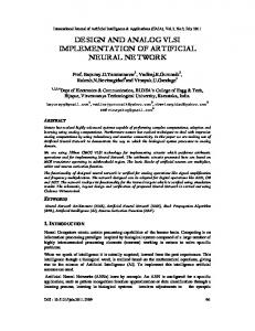
The performance of turbo-code decoder with the RSC code with the octal generator (35, 23) for block length of N = 256, N = 512, and N = 1024 are evaluated. Uniform quantization at the input for all decoders considered is assumed. Figures 5 to 7 illustrate the simulated decoding performance of the rate 1/3 Turbo-code decoder for

Figure 5.

Turbo-code decoder performance (Block length = 256).


49

tised performance. The input wordlength of 4-bits is chosen for the simulations since there is no significant improvement beyond 3-4 bit input wordlength. 4.

VLSI Implementation

At the architectural and circuit levels, the main contribution to power consumption in complementary metal oxide (CMOS) circuits is attributed to the charging and discharging of parasitic capacitors that occur during logical transitions. The average switching energy of a CMOS gate (or the power-delay product) is given by the following equation: Figure 6.

Figure 7.



different data block sizes. As shown in the figures, the performance improves as the size of data block gets larger (i.e., close to 1dB improvement at the bit error rate of 10−5 by increasing the data block size from N = 256 to N = 1024). The predetermined weighting Q factors, obtained from the simulations, are {4, 4, 4, 4}, {4, 4, 4, 2}, and {4, 4, 4, 4} for data block size N of 256, 512, and 1024, respectively. The values in the sets represent each Q at different iterations. It is evident from the figures that the performances does not improve beyond 4 iterations for a particular design. The performance of decoder architecture presented in this paper is inferior to the original decoding algorithm by 1dB coding gain loss. However, the original decoding algorithm often requires more than 10 iterations and a complex σ L2 estimator to achieve adver-

2 Energy/Operation = Caverage · Vsupply

(21)

where Caverage is the average capacitance being 2 is the supply voltage. switched per clock, and Vsupply The quadratic dependence of energy on voltage makes it clear that operating at the lowest possible voltage is most desirable for minimizing the energy per consumption; unfortunately, reducing the supply voltage comes at the cost of a reduction in computational throughput. One way to compensate for these increased delays is to use architectures that reduce the speed requirements of operations while keeping throughput constant. One architectural approach for maintaining throughput with slower circuitry is to use parallelism through hardware duplication. By using identical units in parallel, the speed requirements on each unit are reduced, allowing for a reduction in voltage. This approach is particularly useful for iterative decoding algorithm where the final decision in taken after the multiple iteration of the process. However, duplicating units has limit due to the available silicon area. When the duplication factor becomes large so that multiple chips need to be employed, the power dissipated by the inter-chip communication becomes serious due to large interconnect capacitance. Hence, reduction in the decoder architecture complexity is also beneficial for low power system design. In this section, VLSI implementation of turbo-code encoder and decoder is presented. The turbo-code encoder and decoder are structurally modeled using Verilog hardware description language and the chips are synthesized with the Epoch CAD design environment based on 0.6-µm CMOS standard cell technology. The supply voltage of the chips is set to be 3.3 V. The turbo-code decoder for the data block size N of 256 bits and memory size of 4 are designed. The RSC

50

Hong and Stark

Figure 8. (a) Encoder functional block diagram, (b) Recursive systematic convolutional coder with Trellis termination, (c) Recursive systematic convolutional coder without Trellis termination.

code at the turbo-code encoder is generated by the octal generator function (35, 23). The data rate of 1Mbps is assumed in the discussion. Thus, the Turbo-code decoder accepts Rk = (xk , yk , L k ) every T = 1 µsec. 4.1.

trellis termination required by the first RSC encoder. In this way, the encoder eliminates further latency that exists with one delay line implementation. N − K of N (N = 256 and K = 5 in the implementation) information data bits go into the RSC1/TT (TT stands for Trellis Termination) every T seconds where T represent a data bit interval. Among N bits of a data frame block, only N − K bits are the actual information bits while K bits are for trellis termination. The functional block diagram of the recursive systematic convolutional-code (35, 23) encoders with constraint length of K = 5 is shown in Fig. 8(b) and (c). Additions are accomplished by the modulo-2 sum operations. The convolutional-code encoder for RSC1 (Fig. 8(b)) and RSC2 (Fig. 8(c)) are structurally different in that RSC1 has a integrated trellis termination logic where RSC2 has its trellis left open. 16-states trellis structure corresponding to the code (35, 23) is shown in Fig. 9. The encoded bit is indicated on the transition arcs where solid arcs correspond to input data bit 1 and dashed arcs correspond to input data bit 0. The data interleaver/deinterleaver consists of a synchronous up-counter, a pseudo-random noise (PN) sequence generator, and a static memory block for read write operation. For data interleaving, data memory is written to the block of memory sequentially by the address generated by the synchronous up-counter and read from the block of memory pseudo randomly by the address generated by the PN sequence generator. The PN sequence is generated by shift feedback registers [2]. For data deinterleaver, the order of writing and reading operations is reversed.

Encoder Design

Overall functional block diagram of a turbo-code encoder is shown in Fig. 8(a). The encoder consists of two recursive systematic convolutional encoders and a block of memory for data interleaving operation. Since it takes finite amount of time for interleaving, delay lines are introduced. These sub-components of the turbo-code encoder are controlled by a sequencer. Two delay-line blocks are introduced at the output of both Dk and C1,k for synchronizing with C2,k . The reason that two delay lines are introduced at the output instead of one delay line at the data input is due to

Figure 9.

Trellis structure.


4.2.

Pipelined Multi-Stage Decoder Design

A single iteration of turbo-code decoding process which corresponds to one stage of the pipelined decoder requires two component decoders, Decoder1 and Decoder2, connected in a serial configuration as shown in Fig. 2. The first component decoder, Decoder1, accepts uncoded input xk , coded input y1,k , and extrinsic information L 2,k . The first component decoder generates new extrinsic information L 1,k . The second component decoder, Decoder2, accepts interleaved version of xk , coded input y2,k , and L 1,k which was generated by the first component decoder. The major functions of each component decoder are to compute the branch metric, forward path metrics, backward path metrics, and the extrinsic information. The computation of the metrics is performed by four independent processing units and these units exchange data through the storage memory. 4.3.

51

Component Decoder Design

The functional block diagram of the component decoder is shown in Fig. 10. Branch metric unit (BMU) takes three kinds of input and generates branch metrics. The metric generated by the BMU is stored in the branch metric memory and routed to forward path metric unit (FPMU) simultaneously. Backward path metric unit (BPMU) reads metric stored in the branch metric memory. After processing, its metric is stored in the backward path memory. After both forward and backward path metrics are calculated, LLR calculation unit generates weighted data. For each symbol vector Rk received, 2M branch metrics and 2M forward path metrics are generated where M = 2 K −1 represents the number of states which depend on the constraint length K of the code. After all the branch and forward metrics are generated for N received symbol vectors R, the backward path metrics and extrinsic information are generated corresponding to the completion of one component decoding cycle.

Figure 11.

Branch metric calculation unit.

The metric generation can be accomplished with simple adders and comparators. The latency is 2N (N for branch and forward path metrics and N for backward path metrics and extrinsic information). The maximum throughput obtainable with given circuit implementation is limited by the size of trellis states M because the number of operations in a symbol duration is proportional to the size of trellis state [16]. 4.3.1. Branch Metric Calculation Unit. At each bit time k the Branch Metric Calculation Unit (BMU) takes Rk and generates branch metric γ˜k0 (m) and γ˜k1 (m) for states m = 1, . . . , 32 according to Eq. (19). The functional block diagram of the BMU is shown in Fig. 11. As soon as Rk is received, −Rk is generated. Both Rk and −Rk are applied to four three-input adders. These adders simultaneously generates four possible branch metrics values {a, b, c, d}. Four possible metric values are produced since there are only four combinations in generating the branch metrics (i.e., i ∈ {0, 1} and cm ∈ {0, 1}). Since the total number of branch metrics equals to the number of states in the Trellis, the BMU generates 32 branch metrics (16 γ˜k0 and 16 γ˜k1 ) by shuffling and reusing four metric values. The first shift register which generates γ˜k0 (m) for m = 1, . . . , 16 loads four possible values in parallel in following order [b, a, a, b, a, b, b, a, b, a, a, b, a, b, b, a].

Similarly, the second register which generates γ˜k1 (m) loads in parallel in following order [c, d, d, c, d, c, c, d, c, d, d, c, d, c, c, d].

Figure 10.

Block diagram of the component decoder.

(22)

(23)

The ordering of the metrics corresponds to the state transitions determined by the encoding scheme. These four metric values are loaded at a rate of 1 MHz and shifted out at a rate of 16 MHz. The metric being shifted out is stored in the branch metric memory and

52

Hong and Stark

simultaneously routed to input register of the forward path metric calculation unit. Invert operation is performed by 1’s complement operation eliminating an adder for each invert operation. XOR gates are used for the operation. Four parallel adders are used to lower the speed requirement so that the voltage can be reduced in order to minimize the processing power. The operating speed of the adders depends on the bit rate and the speed of shifting operation depends on the number of states in the Trellis. In this implementation, 16 MHz clock is used to control this shift operation. Figure 13.

4.3.2. Forward Path Metric Calculation Unit. At each state transition time m with in bit time k, the Forward Path Metric Calculation Unit (FPMU) takes branch metrics γ˜k0 (m) and γ˜k1 (m) generated by the 0 (m 0 ) and BMU and the forward path metrics α˜ k−1 1 0 α˜ k−1 (m ) stored in the Forward Path Metric Memory and generates new branch metric α˜ k0 (m) and α˜ k1 (m). Newly generated metrics are stored back to Forward Path Metric Memory. The functional block diagram of the FPMU is shown in Fig. 12. 0 1 (m 0 ) and α˜ k−1 (m 0 ) The previous time metrics α˜ k−1 are compared and the maximum of two is selected. The maximum value is input to both adders. The outputs of adders are the new metrics. The FPMU starts to compute as soon as the first branch metrics (one out of M) are calculated and routed by the BMU. Hence the operation speed of the FPMU is proportional to the total number of states M (i.e., 16 MHz). The clock controlling the FPMU is a half cycle delayed version of the clock controlling the shift register in BMU. The forward path metric memory is dual ported so that both read and write operations are possible.

Figure 12.

Forward path metric calculation unit.

Backward path metric calculation unit.

The forward path metric is calculated Eq. (17) where initial conditions are set to α˜ 0 = 1 and α˜ 0 (m 6= 0) = 0. 4.3.3. Backward Path Metric Calculation Unit. The Backward Path Metric Calculation Unit (BPMU) takes branch metrics γ˜k0 and γ˜k1 stored in the Branch Metric Memory and the backward path metrics β˜k and β˜k stored in the Backward Path Metric Memory and generates new backward path metric β˜k−1 and β˜k−1 . These newly generated metrics are stored back to Backward Path Metric Memory. The functional block diagram of the BPMU is shown in Fig. 13. The operation of BPMU starts as soon as branch metrics for last bit of the data block are calculated by FPMU. The operating speed of the BPMU is also 16 MHz. The forward path metric memory is dual ported so that both read and write operations are possible. The backward path metric is calculated using Eq. (18) where initial conditions are βÑ (0) = 1, βÑ (6=0) = 0 for the first component decoder and initial conditions for the second component decoder are βÑ (m) = α˜ N (m). 4.3.4. LLR Metric Calculation Unit. For each state m, the LLR Metric Calculation Unit (LLRU) takes the forward path metric α˜ k0 and α˜ k1 stored in the forward path metric memory and the backward path metric β˜k−1 and β˜k−1 stored in the backward path metric memory ˜ k and L. The functional and generates two outputs 3 block diagram is shown in Fig. 14. The adders and compare/select units operate at 16 MHz for adding and comparing all M metrics but the subtractors operates at 1 MHz where the output is selected only at the end. The compare/select takes 16 input in serial fashion at a rate of 16 MHz and generates the largest input at a rate


Figure 14.

LLR metric calculation unit.

of 1 MHz. The second subtractor generating L is not active in the last stage of the decoder since the extrinsic information L is no longer needed. The values of LLR are calculated using Eq. (11) and the values of L are calculated using equation 31 =

2L 2 2L 1 + 2x + L 1 , 32 = + 2x + L 2 Q Q

Memory units addressing and organization.

a shuffle block is incorporated to generate A0 , which addresses the state m 0 . Separate memory units are used to store metrics γ˜ 0 and γ˜ 1 . Also α˜ 0 and α˜ 0 use separate memory units. This separation reduces the speed of the address counter by a factor of 2. With this speed reduction, slower memory can be utilized. All the memory units in the decoder are dual-ported for metric read/write operations. Interleaving and deinterleaving operations are the integral part of the overall decoding process. The data interleaver/deinterleaver consists of a synchronous up-counter, a pseudo-random noise (PN) sequence generator, and a static memory block for read write operation. For data interleaving, data memory is written to the block of memory sequentially by the address generated by the synchronous up-counter and read from the block of memory pseudo randomly by the address generated by the PN sequence generator. For data deinterleaver, the order of writing and reading is reversed.

(24)

4.3.5. Memory Units and Addressing. The component decoder accesses various metric memory units extensively throughout the decoding process. Their access patterns depend on the state transitions of the trellis, which is determined by the generator functions of encoding scheme. Figure 15 illustrates the address generation mechanism and the data storage organization respectively. One synchronous counter is used to generate addresses for the BMU and the FPMU, and one additional counter for the BPMU and the LLRU. The address generated by the counter is appropriately latched to handle metric memory access timing. As shown in the figure, an address A, which addresses the state m, is organized as concatenation of two segment, AM and AN, where AN represents the time sequence, AM represents state position, and AS represents the time sequence. Since the destination state position differs from the source state,

Figure 15.

53

4.3.6. Timing. There are three main synchronization clock signals in the architecture. One clock signal controls the time sequence of the decoder that is equal to the data bit time. Each bit time interval is divided into 16 state sequence and each of the state time interval is divided into two for accommodating reading and writing memory units. Thus, the highest clock signal generated by the architecture is equal to 32 times the data bit interval. The timing relationship is shown in Fig. 16. 5.

Evaluations

A low-complexity turbo-code decoder architecture presented in this paper is designed and implemented using standard cell CMOS processing technology. Its decoding performance and hardware complexity for different numbers of iterations and block sizes are evaluated. In addition, various well known decoders for Hamming(7, 4), BCH(31, 16), BCH(31, 21), Golay(23, 12), Hadamard(16, 4), Hadamard(64, 6), convolutionalcode(1/2, 7) are also designed and implemented with the same processing technology and compared with

Figure 16.

Control clock signal for the decoder.

54

Hong and Stark

Figure 17. N = 256).

Turbo-code decoder chip layout (Block length

the turbo-code decoder. For Hamming, BCH, and Golay codes, a hard decision decoding algorithm utilizing a simple syndrome decoding is incorporated. For Hadamard and convolutional-codes, hard decision decoding, as well as soft decision decoding, is designed and implemented. All of the decoders evaluated in this section are designed and implemented using the same processing technology. 5.1.

Decoder Complexity

Figure 17 illustrates the chip layout of the turbo-code decoder implemented using the Epoch CAD design environment based 3.3 V 0.6-µm standard cell technology. The chip size of the turbo-code decoders is dominated by the size of the storage memory used. Even though the power consumed by the memory is not critical, the size of memory may be so large that multiple chips may be required in the implementation. In case of multiple chip decoder, the power consumption will increase dramatically due to the power dissipated to drive large capacitance I/O interconnects connecting the chips. We analyze the required storage memory for the decoders discussed in the paper. Due to interleaving and recursive nature of the turbo-code decoding algorithm, many storage memory modules are required. The size of each memory module depends on the wordlength of various inputs, metrics, trellis size, and the data frame size. For single iteration of the decoder, the required memory consists of the branch metric memory, forward

Figure 18.

Decoder chip size of various decoders.

and backward path metric memory, extrinsic information memory, interleaver, deinterleaver, and input delay buffer. Thus, total memory size can be expressed as MEM = 3N + 4N W L + 2N Win + 4N M Wγ˜ + 4N M Wα˜ + 2N M Wβ˜

(25)

where N represents the size of data block, M represents the number of states in the trellis, Winput represents wordlength of the inputs, Wγ˜ represents wordlength of the branch metric, Wα˜ represents wordlength of the forward path metric, Wβ˜ represents wordlength of the backward path metric, and W L is the wordlength of the extrinsic information. Figure 18 illustrates the chip sizes of the turbocode decoders as well as the well-known decoders considered in this paper. The block decoders such as Golay(23, 12) and BCH(31, 16) require considerable amount silicon area due to codewords storage. In contrast, Hadamard decoders require relatively smaller silicon area. Among all of the decoders considered, turbo-code decoders require large amount of silicon area due to the multiple copies of decoder processing units and storage. When the chip size is excessive, time sharing architecture may be needed to reduce the overall chip size. 5.2.

Decoder Performance-Power Relationships

The relationship between the estimated power consumption and the performance is an important measure of the decoders when the power is the main concern in the design.


Figure 19. Decoding performance vs. power consumption at BER = 10−3 .

is comparable to the power consumption of the conventional convolutional-code decoders. For example, the performance of the turbo-code decoder was better than that of the Viterbi decoder for convolutional-code by more than 1dB at the BER of 10−3 and 2 dB at the BER of 10−5 . Even with 2 iterations, the performance improvement is significant while the power consumption is only doubled. Also shown in the figures, one can draw an imaginary line connecting the points that signifies the power consumption and performance bound. Most decoders not indicated in the Figs. 19 or 20 fall within the upper region of the bounds indicating that such decoders are not power efficient choice for low energy communications system. The relationship curve between the performance and the power consumption is seamlessly extended by the low-complexity turbo-code decoders. However, one important information missing from this plot is that the plot does not illustrate the amount of power incurred in modulator/demodulator due to different code rates among decoders. For low code rate, it is certain that the more power is dissipated in the other parts of communication systems rather than the decoder itself. 6.

Figure 20. Decoding performance vs. power consumption at BER = 10−5 .

Figures 19 and 20 illustrate the power and performance relationship of decoders including the turbocode decoder at different bit error rate (BER) requirements. The power consumptions for the decoders are obtained from the implementation based on the standard cell library with the supply voltage fixed at 3.3 V. The reference information data rate of 1Mbps is assumed for all decoders. Thus, the power consumption of the decoders can be further reduced by optimizing at the circuit level and by scaling the supply voltage for the given information data rate. Figures 19 and 20 also illustrate that the performance of the turbo-code decoder is generally better than that of the other type of decoders while the power consumption of the low-complexity turbo-code decoders

55

Conclusion

Channel coding is commonly incorporated to obtain sufficient reception quality in wireless mobile communications transceiver to counter channel degradation due to intersymbol interference, multipath dispersion, and thermal noise induced by electronic circuit devices. For low energy mobile wireless communications, it is highly desirable to incorporate a decoder which has a very low power consumption while achieving a high coding gain. In this paper, a sub-optimal low-complexity multi-stage pipeline decoder architecture for a powerful channel coding technique known as “turbo-code” is presented. The presented architecture avoids complex operations such as exponent and logarithmic computations. The turbo-code decoding algorithm is reformulated for an efficient VLSI implementation. Furthermore, the communication channel statistic estimation process has been completely eliminated. The architecture has been designed and implemented with the 0.6 µm CMOS standard cell technology using Epoch computer aided design tool. The performance and the circuit complexity of the turbocode decoder are evaluated and compared with the other types of well-known decoders. The power

56

Hong and Stark

consumption of the low-complexity turbo-code decoder is comparable to that of the conventional convolutional-code decoder. However, the low-complexity turbo-code decoder has a significant coding gain over the conventional convolutional-code decoders and it is well suited for very low power applications. Acknowledgments This research was supported by the Department of Defense Research & Engineering (DDR&E) Multidisplinary University Research Initiative (MURI) on “Low Energy Electronics Design for Mobile Platforms” and managed by the Army Research Office (ARO) under grant DAAH04-96-1-0377.

16. Sangjin Hong and Wayne E. Stark, “VLSI design and implementation of low-complexity adaptive turbo-code encoder and decoder for wireless mobile communication applications,” Proc. SiPS98, 1998. 17. S. Benedetto and G. Montorsi, “Design of parallel concatenated codes,” IEEE Transactions on Communications, pp. 591–600, 1996. 18. S. Benedetto, D. Divsalar, G. Montorsi, and F. Pollara, “Softinput soft-output modules for the construction and distributed iterative decoding of code networks,” European Transactions on Telecommunications, Vol. ETT9, 1998. 19. Joachim Hagenauer, Elke Offer, and Lutz Papke, “Iterative decoding of binary block and convolutional codes,” IEEE Transactions on Information Theory, pp. 429–445, 1996.

References 1. J.G. Proakis, Digital Communications, McGraw-Hill, 1995. 2. R.C. Dixon, Spread Spectrum Systems with Commercial Applications, Wiley Interscience, 1994. 3. A.J. Viterbi, CDMA: Principles of Spread Spectrum Communication, Addison-Wesley, 1995. 4. C.E. Shannon, “A mathematical theory of communications,” Bell System Technical Journal, Vol. 27, pt. I, pp. 379–423; pt. II, pp. 623–656, 1948. 5. A.J. Viterbi, “Error bounds for convolutional codes and an asymptotically optimum decoding algorithm,” IEEE Transactions on Information Theory, Vol. IT-13, pp. 260–269, 1967. 6. J.K. Omura, “On the Viterbi decoding algorithm,” IEEE Transactions on Information Theory, Vol. IT-15, pp. 177–179, 1969. 7. G. Fettweis and H. Meyr, “High-speed parallel Viterbi decoding: Algorithm and VLSI-architecture,” IEEE Communication Magazine, Vol. 29, pp. 46–55, 1991. 8. P.J. Black and T.H. Meng, “A 140-Mb/s 32-state, radix-4 Viterbi decoder,” IEEE Journal of Solid-State Circuits, Vol. 27, pp. 1877–1885, 1992. 9. B.K. Min and N. Demassieux, “A versatile architecture for VLSI implementation of the Viterbi algorithm,” Proc. ICASSP, 1991, pp. 1101–1104. 10. C. Berrou, A. Glavieux, and P. Thitimajsima, “Near Shannon limit error-correcting coding and decoding: Turbo-codes (1),” Proc. ICC, Geneva, 1993, Vol. 2, pp. 1064–1070. 11. P. Robertson, “Illuminating the structure of code and decoder of parallel concatenated recursive systematic (Turbo) codes,” in IEEE Global Telecommunications Conference, Vol. 3, 1994. 12. L.R. Bahl, J. Cocke, F. Jeinek, and J. Raviv, “Optimal decoding of linear codes for minimizing symbol error rate,” IEEE Transactions on Information Theory, Vol. IT–20, pp. 248–287, 1974. 13. Comatlas, Chateaubourg, France, “CAS 5093 Turbo-Code Codec, Data sheet,” August 1994. 14. Efficient Channel Coding, Inc., Eastlake OH, USA, “ECC Turbo product code technology,” March 1998. 15. Small World Communications, Adelaide, Australia, “MAP04 and MAP04A 16 State MAP Decoders,” April 1998.

Sangjin Hong received the B.S. and M.S. degrees in EECS from the University of California, Berkeley in 1985 and 1992 respectively. He is currently a Ph.D. candidate in the Department of Electrical Engineering and Computer Science at the University of Michigan, Ann Arbor. He has worked at the Ford Aerospace and Communications Corporation in Sunnyvale California from 1985–1989 where he was involved in developing computer systems for the satellite communications system. He has also worked at Samsung Electronics Corporation in Korea as a technical consultant where he developed DSP hardware systems for the military tank target acquisition system. He also provided weekly seminar to the engineers in the company. His current research interests are in the areas of low power DSP and wireless communication system design and performance evaluation. He worked on various VLSI decoder architecture optimizations for low-power applications. [email protected]

Wayne E. Stark received the B.S. (with highest honors), M.S., and Ph.D. degrees in electrical engineering from the University of Illinois, Urbana in 1978, 1979, and 1982 respectively. Since September 1982


he has been a faculty member in the Department of Electrical Engineering and Computer Science at the University of Michigan, Ann Arbor where he is currently Professor. From 1984–1989 he was Editor for Communication Theory of the IEEE Transactions on Communication in the area of Spread-Spectrum Communications. He was involved in the planning and organization of the 1986 International Symposium on Information Theory which was held in Ann Arbor, Michigan. He was selected by the National Science Foundation as a

57

1985 Presidential Young Investigator. He is principal investigator of a Army Research Office Multidisciplinary University Research Initiative project on Low Energy Mobile Communications. His research interests are in the areas of coding and communication theory, especially for spread-spectrum and wireless communication networks. Dr. Stark is a member of Eta Kappa Nu, Phi Kappa Phi and Tau Beta Pi and a Fellow of the IEEE. [email protected]