trained on-chip with a simplijed variant on reinforcement learning. 1 Introduction ... tion orders l through 3, giving rise to some novel modu- .... table from a binary address-encoded representation of the ... sinusoidal input with amplitude 0.5 and period 128. ..... Mixed-Signal RAM Decision-Feedback Equalizer for Disk. Drives ...
Design and VLSI Implementation of an Adaptive Delta-Sigma Modulator Gert Cauwenberghs * Dept. of Electrical and Computer Engineering The Johns Hopkins University Baltimore, MD 2 1218-2686 E-mail: gert@jhu .edu Abstract The quality and stability of noise shaping is a concern in the design of higher-order delta-sigma modulators for high-resolution, high-speed oversampled analog-to-digital conversion. We reformulate noise-shaping modulation alternatively as a nonlinear optimal control problem, where the objective is tofind the binary modulation sequence that minimizes signal swing in a cascade of integrators operating on the difference between the input signal and the modulation sequence. We use reinforcement learning to adaptively optimize a nonlinear neural classijec which outputs modulation bits from the values of the input signal and integration state variables. Analogous to the classical pole balancing control problem, a punishment signal triggers learning whenever any of the integrators saturate. We train a simple classiJer consisting of locally tuned, binary address-encoded neurons to produce stable noise shaping modulation, and present experimental results obtainedfrom analog VLSI modulators of orders one and two. The integrated classijier contains an array of 64 neurons trained on-chip with a simplijed variant on reinforcement learning.
-1-4
Figure 1: Noise-shaping modulators for oversampled A/D conversion. (a)First-order delta-sigma modulator. (b)Generalized higher-order structure with nonlinear classifier. All operations are sampled, discrete-time. (signal swing) of the integration variables. As we will show, this is equivalent to minimizing the low-frequency in-band quantization noise of the modulator. The control problem in our formulation has strong similarities with the pole balancing problem, solved efficiently using reinforcement learning [2]. The objective of the work presented here is not a highperformance delta-sigma modulator circuit design per se, but to demonstrate the feasibility of integrating adaptive functions in the classifier, for the purpose of improving performance through a simple control criterion. It may seem counter-intuitive that adding more analog circuit complexity to the design of a delta-sigma modulator could improve rather than degrade performance, due to increased sensitivity to noise and process parameters. In the case considered here, the additional circuitry does not affect the analog signal path, but affects the quantized output only. By replacing the quantizer by a more sophisticated nonlinear classifier that adapts to the statistics of the signal, noise-shaping properties are improved and less quantization noise leaks into the signal frequency band. We first define noise-shaping modulation in the nonlinear control framework, and then formulate reinforcement learning as applied to the optimization problem. Next, we present results on training a simple binary address-encoded classifier to produce noise-shaping modulation of integration orders l through 3, giving rise to some novel modulation structures. Finally, we present experimental results
1 Introduction Noise-shaping modulation architectures such as deltasigma modulators are attractive for high resolution oversampled A / D (analog-to-digital) data conversion [ I], trading bandwidth of a fast, low-resolution converter for improved resolution by oversampling and modulating the signal to push quantization noise out of the signal band. Higher-order delta-sigma modulators offer high resolution at significantly increased signal bandwidths (lower oversampling ratios); however, they are prone to instabilities for orders beyond two. Most higher-order noise-shaping architectures considered so far are direct linear extensions on the standard first-order delta-sigma modulator, shown in Figure 1 (a). We approach noise-shaping modulation alternatively as a nonlinear control problem, where the binary modulation sequence controls a “plant” which consists of a cascade of integrators that operate on the quantization error, i.e., the difference between analog input and binary modulation sequences, shown in Figure 1 (b). The optimal modulation sequence is defined as the one which minimizes the energy ‘This work was supported by NSF under Career Award MIP-9702346 and by ARPNONR under MURI grant “14-95-1-0409. Chip fabrication was provided through MOSIS.
155 1063-9667197$10.00 0 1997 IEEE
I
on an analog VLSI modulator comprising a cascade of integrators and an array of 64 locally tuned, address-encoded neurons with on-chip learning on a 2 pm CMOS chip.
objective becomes equivalent to that in multi-segment pole balancing: control the movement of a cart y ( t ) driving a multi-segment pole under gravity such as to maintain the segments upward along the vertical axis, trying to confine segment excursions xi ( t )within limits of stability.
2 Nonlinear Noise-Shaping Modulation We state noise-shapingmodulation for oversampled A/D conversion as an optimal nonlinear control problem. The order-n modulator comprises a cascade of n integrators z , ( t ) operating on the difference between the analog input u ( t ) and the binary ( f l ) modulated output y ( t ) , Figure 1 (b):
+
3 Reinforcement Learning Reinforcement learning techniques are applicable to general learning tasks defined by a discrete, delayed, external reward or punishment signal r ( t ) which serves as the only indication of performance available for training [2], [3], [4], [5]. The classical example where reinforcement learning is applied is the pole-balancing problem, which it efficiently solves [2]. Similarly, in the context of noiseshaping modulation, we use a failure signal, indicating saturation in one or more of the integrators, to reinforce stability of noise-shaping. A nonlinear neural classifier, depicted in the box labeled “NN’ in Figure 1 (b), produces the modulation sequence from the state of the input and integrators, y ( t ) = f ( u ( t ) :xi(t>). Similar to the “boxes-system” used in [2], the classifier chosen here has locally tuned, hardthresholding neurons, effectively implementing a look-up table from a binary address-encoded representation of the statc space spanned by u ( t ) and :c,(t). In particular, y ( t ) = yx(t) where y(t) is the index of the address selected from address bits generated from the sign of the components u ( t ) and zi(t):
+
1) = q ( t ) a ( u ( t )- y(t)) (1) z;(t+l) = z;(t)+az,-l(t), i = 2 ? . . . r ~
zl(t
with modulation gain U. = 0.5. Notice that this choice of noise-shapingfiltering through successive integration is not critical, and the cascade of filters in (1) can be replaced by a bank of filters, of which the last one has n poles located near 2 = 1. For generality, denote the z-transforms of the n, filters as H;(z), with - Y ( Z ) ) > i = 1 , . . .n
(2)
Y ( z ) = U ( Z )- H;-’(z) X ; ( z ) , ,i = l ? . . . n .
(3)
Xi(.) = Hi(.) (U(.) or, equivalently
The second term in (3) represents the error in quantizing U(.) as Y ( z ) . The effect of noise shaping is apparent from the high-pass nature of the noise transfer function (NTF) Hi-‘(z), shaping the noise spectrum X;(z) to push low-frequency components outside of the signal band. Although this is the same NTF as appears in linear analysis of the delta-sigma modulator [ 11, where it shapes quantization noise, we are not making any assumptions on explicit use of a quantizer. Rather, noise is considered as being contributed directly by the amplitude of the integration state variable IC; ( t) . The control objective is to choose the binary sequence y ( t ) such as to minimize the energy of the state variables lza(t)I2 over time. This corresponds to minimizing the power spectrum of the noise = ejwT)I2near zero frequencies, z M 1. This in turn yields a modulation output Y (2) which most faithfully represents the input signal I;(2) at lower frequencies, i.e., in the signal band. Preference among components i in the minimization of lzi(t)I2is givcn to the last stage in the cascade, i = n, which yields noise shaping of the highest order n. The reason for still including the n - 1 intermediate integration variables is because a cascade of integrators easily saturates for even small perturbations of the input. Saturation of the i-th integrator causes instability of noise shaping at order i , leading to cancellation of the zero in the NTF in (3) at zero frequency ( z = 1). By still minimizing the preceding integrators in the chain, xj ( t )with j < i, stability of noise shaping is enforced at least at a lower order, and at worst at order one (j= 1). Because of the natural tendency of the integrators to saturate, minimizing lxi(t)1* is almost equivalent to simply constraining the excursion of the integration variables within saturation limits, Iz;(t)l< zSat.Then the control
U+(t) = sign(u(t)) X i + ( t ) = sign(.r,(t)). i = l . ” . n , .
(4)
This simple choice of input representation is by no means designed to be optimal, but serves as a proof of principle, transparent for interpretation and suited to implementation in VLSI. Still, this representation is powerful enough to produce first-order and second-order noise shaping as illustrated below. As in [2], a “reward” signal r ( t ) is generated, equal to zero as long as the modulator is stable, and -1 for punishment when failure occurs (saturation of one or more integrators). To reinforce past actions y(t) of the network leading to future reward r ( t ) ,an “adaptive critic element” q ( t ) is trained along with the network to predict the future reward from the present state of the network. Similar to the classifier y ( t ) , the adaptive critic q ( t ) is implemented as a look-up table q ( t ) = q x ( t )with identical address encoding ~ ( tof)the state space. We reformulate reinforcement learning defined in [2] as follows. Let Y k and q k be the adaptive parameters of the classifier and adaptive critic, and let ek denote the “eligibility” traces of the corresponding neurons. Then the parameter updates are given by:
Ix~(z
Uk(t 4k(t
+ 1) + 1)
= Yk(t) + a T^(t)erc(t) Y k ( t )
+
(5)
= qk.(t) P T^(t)Q ( t ) where the internal reinforcement ?(t)is constructed as
+
?(t)= r ( t ) Y q ( t ) - q(t - 1) and the eligibilities e6 ( t )are updated as ek(t
156
+ 1) =
X ek(t) = Aek(t)
+ (1 - A)
(6)
k =~ ( t ) otherwise (7)
Table 1: Trained values y k for n = 1.2.
l0.F"'
U+
XI+
X2+
0 0
0 1
8
1 1
0 1
0 1
'
'
JJ
y
(ri=I)
8 P P
0
"""'
'
1 0 1
"""'
(ri=2)
t
'
'
" " "
'
'
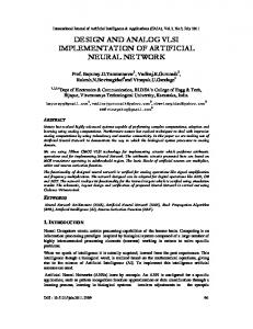
""'J Figure 3: Chip micrograph. Top: array of reinforcement learning neuron cells. Bottom left: cascade of integrators. Bottom right: state space address encoding.
d
IO4
10
'
10
10
'
We have tried to generate third-order noise-shaping with the same state space encoding (4) for n = 3, but failed to get stable and consistent results. We attribute this to the coarse encoding, and note that satisfactory results have been obtained for n = 3 using a neural classifier with continuous distributed representation, trained through a perturbative version of reinforcement learning [6].
.
IO0
Normalized Frequency (units 1/T)
4 Analog VLSI Implementation 4.1 System Level Architecture
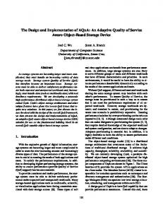
Figure 2: Simulated output modulation spectra of the trained noise-shaping modulators of orders 'n, = 1 2 for a sinusoidal input with amplitude 0.5 and period 128. ~
We have integrated a cascade of 6 integrators, an 11-bit address state encoder, and an address-encoded classifier with 64 reinforcement learning neurons on a 2.2 mm x 2.2 mm chip in 2 pm CMOS technology. A micrograph of the VLSI chip is shown in Figure 3. Although of limited use as presently implemented for demonstration purposes, this chip is to our knowledge the first analog VLSI implementation of delayed reinforcement learning embedded in a real-time application. Reinforcement learning in a digital VLSI framework is described in [7], and related work on instinct-rule learning in an analog neural classifier for robot navigation is presented in [SI. The bank of cascaded integrators xi ( t )is implemented using fully differential switched-capacitor circuits. The state encoder contains a bank of comparators and logic to encode the state of the input signal and integration variables u ( t ) and xt(t),assigning one sign bit and one amplitude bit to each variable, except no amplitude bits for zs(t)and zg(t). Each sign bit encodes polarity as in (4). Each amplitude bit encodes a threshold on the absolute signal level, a feature which we did not use in the experiments reported here. Selected bits from the state encoding are used to address the input space of the classifier. The classifier implements a network of 64 neurons with locally tuned input response, as defined above. For convenience of implementation, the neuron cells are arranged in an 8 x 8 2-D array as in a RAM, activated through 3 vertical and 3 horizontal address bit lines.
with ~ ( tthe) index of the address selected according to (4). The results of applying reinforcement learning to a classifier to stabilize a cascade of one and two integrators are listed in Table 1 and illustrated in Figure 2. The learning constants used in the simulations were a = 0.5, D = 0.01, 7 = 0.9 and X = 0.8. During training, the input ~ ( was t) presented 4,092 random samples uniformly distributed in the [ O S . . .0.5] interval. Because of the simple functional form of the classifier (4), we can easily interpret its structure from the values of its parameters at learning convergence, listed in Table 1. For n = 1, information on the polarity of the input (U+) is deemed irrelevant, and the classifier reduces to a one-bit quantizer y X: as in the standard first-order delta-sigma modulator. For n = 2, we apparently obtain a novel structure that uses the available information on the polarities U+, X t and X t in the following way:
1 -1 = U+
y(t) = =
"(:Xi=
1
x, -x, = -1
(8)
otherwise.
With no more information on u ( t ) and ~ ( tavailable ) to the classifier, this policy is indeed most sensible in order to minimize risk of future saturation of the integrators. The output modulation spectra produced by the trained noise-shaping modulators of orders n = 1.2 for a sinusoidal input u ( t ) with amplitude 0.5 and period 128 are shown in Figure 2. The different orders of noise shaping are apparent from the noise spectrum at lower frequencies.
4.2 Reinforcement Learning Cell Figure 4 shows the circuit schematic of the reinforcement learning neuron cell, measuring 100 x 130 pm2 in 2 pm CMOS technology. For a compact and robust implementation, the cell implements the reinforcement learning
157
,-
+ SELhor HYST
f
0
32
16
48
64
Address
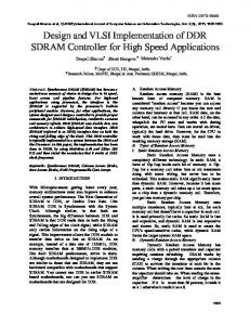
Figure 5: Profile of eligibility time interval across the array of reinforcementlearning cells, measured for different values of 6as set by v6.A one-time address selection marks the start of the interval.
+ SELhor
Figure 4: Circuit diagram of neuron cell with embedded reinforcement learning.
signal, and is constructed externally based on (6). The binary punishment signal r ( t ) is obtained on-chip from saturation detectors in the integrator circuitry, and is activelow when any integrator i n, saturates.
0, triggered by selection of address k , is shown in Figure 5 for all 64 cells as a function of the bias setting v6. Characteristic measurements of the learning rate CY (or, equivalently, the update latency time) are given in Figure 6 , which shows the time intervals between consecutivetoggles of the binary Y k parameter, during continuously eligible negative reinforcement(UPDk ( t )G 1),and with hysteresis enabled. Note the large asymmetry in the update latency time in the ’0’ and ’ 1’ state of yk , due to asymmetries in the circuit and its operation. This is easily alleviated in practice by setting Vapat a larger current bias than Van, although this is not important for learning to be successful. The relatively large variance of the measured 5 and CY parameters across cells can be attributed to transistor current mismatch. This level of variance is typical of minimum size devices, and its effect does not present a significant problem. Figure 7 further illustrates the implemented reinforcement learning mechanisms. Shown are the responses of y ( t ) and q ( t ) under periodic activation of an impulse reinforced punishment ( P ( t ) = - 1) while synchronously cycling the input address ~ ( tthrough ) the 64 neuron cells in sequence, at a rate of 100 psec per cell. As is evident from Figure 7, the credit assignment mechanism of reinforcement learning identifies those cells k which are active during a time interval immediately preceding the punishment, and updates only these parameters yk and q k under
where the auxiliary variable UPDk ( t )is constructed as UPDk(t) = -.^(t)
= o
>0 otherwise ek(t)
(10)
and where hyst(.) in (9) denotes optional hysteresis in the dynamics of yk: hyst(yk) yk when yk retains the same polarity as in the previous update, and hyst(yk) sign(yk) when the polarity of yk flips in the present update. The reason for including hysteresis in the updates of Y k is to avoid oscillations around zero that may arise under repeated presentation of negative reinforcement, and to reduce the effect of leakage in volatile storage during training. The eligibility is given as
=
e k ( t + 1) = =
1 ek(t)
-6
k =X(t> otherwise.
(11)
The net effect of the changes in (9)-(11) with respect to (5)-(7), besides hysteresis in the learning dynamics, is that a cell remains equally “eligible” over a fixed time interval after it is selected, as opposed to an exponential decay of eligibility over time through low-pass filtering (7). The learning updates are provided by a charge-pump circuit virtually free of switch injection noise, described in [6]. The values of the learning constants 6, CY and ,6 are set through global voltages v6,Vanand Vap,biased in the subthreshold MOS region along with auxiliary biases Vbn and Vbp. The reinforcement in (10) is presented to all cells as a binary active-low = - 1) pulse-code modulated
158
I
y=I->O 1
I--
YO0 0
16
32
Address
48
64 0
Figure 6: Time between hysteretic y k updates, across the array of reinforcementlearning cells, measured for different values of (3y as set by Van (and Vap).A single 20 psec negative reinforcement pulse is applied once every cycle.
100
300
200
Time t (unitsT)
400
500
Figure 8: First-order modulator experiments: recorded dynamics of state variables and parameters during on-chip learning.
I 10
Figure 7: Oscillogram of ? ( t ) (top), q k ( t ) (center) and y k ( t ) (bottom) waveforms under periodic impulsive reinforcement. See text for explanation.
20
30
Trial Number
40
50
Figure 9: First-order modulator experiments: failure intervals recorded for 5 learning sessions from random initial conditions.
the external reinforcement. When activated, Y k steadily changes polarity, and q k remains low. Clearly, in an embedded application, the sequence of selected states ~ ( tis)not fixed but adapts together with the policy yk, and the parameters y k and q k settle rather than oscillate as the learning converges (i.e.,as punishment occurs less frequently). This is demonstrated below for the purpose of noise-shaping modulation.
during one learning session are given in Figure 8, showing convergence after roughly 150 input presentations. The time step in the experiments was T = 2.5 msec, limited by the bandwidth of the instrumentation equipment in the recording. The learned pattern of y k conforms to that for n = 1 in Table 1. Learning succeeded at various values of the learning constants 5 and cy, affecting mainly the rate of convergence. Figure 9 shows a record of the time interval between failure in consecutive trials, for 5 different learning sessions, each from random initial conditions of the parameters y k . As in [2], the displayed time intervals in Figure 9 are numerically averaged over consecutivetrials. In most of the cases, convergenceis reached in less than 25 trials, i.e., with fewer than 25 parameter update cycles. At convergence, failures still persist, although at a scale of several thousand time steps T . The persistence of failures at convergence is due to the volatile capacitive storage of yk which causes the
5.2 First-Order Noise Shaping Modulation Test results on training the classifier on-chip to produce noise shaping modulation of order n = 1 using the first integrator are shown in Figures 8 and 9. With hysteresis enabled in (9), this fairly simple learning task can be solved without the adaptive critic ( q ( t ) 0), and accordingly we set F ( t ) r ( t ) . As in the simulations above, the input sequence U ( t )during training is uniformly random with half full-scale maximum amplitude (1 V pp), and the integrator variables xi(t) as well as the eligibilities e k ( t ) are reset to zero after every occurrence of failure, r ( t )= - 1. The dynamics of the state variables and parameters recorded
159
a perturbative stochastic version of reinforcement learning [6]. Further improvements, for orders n = 4 and beyond, require both more advanced training techniques such as variants on heuristic dynamic programming using gradient estimation and prediction in the state space [ 5 ] , as well as careful design of the modulator transfer functions Hi(.) in (2) as a compromise between quality and stability of noise shaping. Besides their efficient implementation in VLSI, the design of such architectures remains an open issue. Similar principles as the ones presented here for noiseshaping modulation can be applied to problems in communications and pattern recognition that call for adaptive control, with less exacting stability requirements than a bank of integrators, for which a simple VLSI approach as demonstrated here may be more than appropriate. Examples can be found in adaptive nonlinear predictive speech coding, and decision-feedback disk drive read inter-symbol interference equalization [9].
c
yo10 yo01 YOW 1
200
400
600
800 1000 1200 1400 1600 1800 2000
Time t (units T)
Figure 10: Second-order modulator experiments: recorded dynamics of the classifier parameters yk ( t )and reinforcement signal r ( t ) during on-chip learning.
References [ 11 J.C. Candy and G.C. Temes, “Oversampled Methods for N D and D/A Conversion,” in Oversampled Delta-Sigma Data Converters, IEEE Press, pp 1-29, 1992.
correct values to decay and drift in absence of reinforcement, triggering failure each time one of the components yk reverses polarity.
[2] A.G. Barto, R.S. Sutton, and C.W. Anderson, “Neuronlike Adaptive Elements That Can Solve Difficult Leaming Control Problems,” IEEE Transactions on Systems, Man, and Cybemetics, vol. 13 (3,pp 834-846, 1983. [3] R.S. Sutton, “Learningto Predict by the Methods of Temporal Differences,”Machine Learning, vol. 3, pp 9-44, 1988.
5.3 Second-OrderNoise Shaping Modulation Results on training the classifier to stabilize two stages of the integrator bank to produce noise-shaping modulation of order two are represented in Figure 10. Convergence is reached in about 1,400cycles, which is a factor three slower than in the case n, = 1. Learning experiments over longer time intervals ( lo7 cycles) show that the mean time between failures is about 500 cycles. When the parameters yk are frozen after convergence (by activating the LOCK switch in Figure 4), the time between failures peaks at lo5 cycles, and varies with the particular input sequence u ( t ) .
[4] C. Watkins and P. Dayan, “Q-Learning,’’Machine Learning, vol. 8, pp 279-292, 1992. [5] P.J. Werbos, “A Menu of Designs for ReinforcementLearning Over Time,” in Neural Networks for Control,, W.T. Miller, R.S. Sutton and P.J. Werbos, Eds., Cambridge, MA: MIT Press, 1990, pp 67-95. [6] G. Cauwenberghs, “Analog VLSI Stochastic Perturbative Leaming Architectures,”to appear in Int. J. Analog Integrated Circuits and Signal Processing, March 1997.
6 Conclusions We reformulated noise-shaping modulation for oversampled A/D conversion as a nonlinear control problem with solutions that are stable for higher orders TL using an optimization criterion directly on the values of the integration variables. The linear thresholding classifier commonly used in delta-sigma modulation is replaced by a more general nonlinear classifier. We applied reinforcement learning to train a nonlinear classifier which uses information only on the polarities of the input and integration variables of the modulator, achieving stable noise shaping of orders n = 1 and 2. Finally, we implemented the adaptive modulator including neural classifier and reinforcement learning on a single analog VLSI chip, and presented experimental results on training the system as first-order and second-order noiseshaping modulators. The remaining challenge is to increase the effective order of noise shaping that can be obtained with an experimental system beyond n = 2 , requiring a classifier of more refined structure than we considered here. We note that simulations support satisfactory results for order n = 3 using a distributed continuous neural classifier, trained with
[7] T.G. Clarkson, C.K. Ng and Y. Guan, “The PRAM: An Adaptive VLSI Chip,”IEEE Trans. on Neural Networks, vol. 4 (3), pp 408-412, 1993. [8] G. Jackson and A.F. Murray, “Competence Acquisition in an Autonomous Mobile Robot using Hardware Neural Techniques,” in Adv. Neural Information Processing Systems, Cambridge, MA: MIT Press, vol. 8, pp. 1031-1037, 1996. [9] B.C. Rothenberg, J.E.C. Brown, P.J. Hurst and S.H. Lewis, “A Mixed-Signal RAM Decision-Feedback Equalizer for Disk Drives,” IEEE J. Solid-state Circuits, vol. 32 ( 5 ) , pp 713-721, 1997.
160