Vol. 14 no. 1 1998 Pages 81-91
BIOINFORMATICS
Design and implementation of a qualitative simulation model of λ phage infection Karsten R. Heidtke and Steffen SchulzeĆKremer MaxĆPlanckĆInstitute for Molecular Genetics, Ihnestraße 73, Department Lehrach, DĆ14195 Berlin, Germany Received on September 29, 1997; revised on December 4, 1997; accepted on December 4, 1997
Motivation: Molecular biology databases hold a large number of empirical facts about many different aspects of biological entities. That data is static in the sense that one cannot ask a database ‘What effect has protein A on gene B?’ or ‘Do gene A and gene B interact, and if so, how?’. Those questions require an explicit model of the target organism. Traditionally, biochemical systems are modelled using kinetics and differential equations in a quantitative simulator. For many biological processes however, detailed quantitative information is not available, only qualitative or fuzzy statements about the nature of interactions. Results: We designed and implemented a qualitative simulation model of λ phage growth control in Escherichia coli based on the existing simulation environment QSim. Qualitative reasoning can serve as the basis for automatic transformation of contents of genomic databases into interactive modelling systems that can reason about the relations and interactions of biological entities. Availability: The general qualitative simulator QSim, written in Lisp, is for research purposes available at http://www.cs.utexas.edu/users/qr/QR-software.html. Our code for the simulation of λ phage growth can be obtained from http://cogito.rz-berlin.mpg.de/qr.html. Contact:
[email protected] or http://igd.rz-berlin.mpg.de/∼steffen.
Introduction Computer-based modelling, simulating and reasoning about biological processes has become of greater interest to biologists. In combination with appropriate software the contents of many molecular biology databases could be translated into special simulation software that deduces behaviour from static, interconnected facts. Thus the myriad facts of functional genomic analyses could be coherently assembled to provide an animated, interactive representation of complex biological systems that can be used to accurately retrieve far reaching interactions between biological entities and to investigate the dynamic behaviour of complex biological systems. The implementation of this scenario faces several severe conceptual difficulties, e.g. the semantic inE Oxford University Press
tegration of heterogeneous, autonomous databases (SchulzeKremer, 1997) and the representation and use of large scale quantities of incomplete and fuzzy biological data. Nearly all of the many existing simulation packages require the users to specify their models in precise, numerical terms. For biologists this is a handicap since there is a large amount of mainly qualitative information emerging from genome mapping and functional genomic experiments that can not be included into numerical kinetic simulations. Even in those cases where e.g. concentrations or enzymatic activities are known those numbers come with a considerable variance. To be able to handle qualitative information for simulation tasks qualitative reasoning has been invented (Forbus, 1984; Kuipers, 1986) and since then been shown to be a powerful method in the domains of medicine (Kuipers and Kassirer, 1987) and qualitative physics (Weld and de Kleer, 1990). Coarsely, the work done in qualitative reasoning about biological systems can be grouped into modelling and reasoning on the one hand (Kazic, 1993a, 1993b; Karp and Mavrovouniotis, 1994) and modelling and simulation on the other (McAdams and Shapiro, 1995; Meyers and Friedland, 1984; Schulze-Kremer, 1990, 1995). Related work on qualitative reasoning in medicine has been done by (Artoli et al., 1996) but no qualitative simulation of a whole biological organism has been completed yet. The control of gene regulation in Escherichia coli (Figure 1) is one of the best understood systems in molecular biology (Ptashne, 1986). We built a qualitative simulation model of the lysogenic and lytic pathway to demonstrate how qualitative reasoning can be applied to problems in molecular biology. In contrast to previous works, we explicitly represent the following interacting compounds in an infected E.coli bacterium: (i) λ phases inside and outside the cell, (ii) viral DNA, (iii) ribosomes, mRNA and proteins, (iv) binding rate of polymerase to promoters, (v) rate of transcription, (vi) rate of translation, (vii) rate of anti-termination by N and Q proteins, (viii) degradation of proteins and mRNA.
81
K.R.Heidtke and S.Schulze-Kremer
Fig. 1. A qualitative description of the different stages realized in our model of λ phage growth control. Solid arrows show extent of transcription, dotted lines represent translation of mRNA, dashed lines indicate protein–DNA interactions.
Systems and methods There are several tools for simulation using qualitative reasoning (Dague, 1995): QSim 4.0 Alpha based on qualitative differential equations (Kuipers, 1994) and the Qualitative Process Engine (QPE) (Forbus, 1990), based on qualitative process theory (Forbus, 1984). QPE is a tool for qualitative reasoning using domain and scenario descriptions. The interaction between objects is defined by processes. Another tool is QPC (Crawford et al., 1990), which compiles QPE’s domain and scenario models into QSim’s qualitative differential equations. QSim is implemented in Common LISP (Steele, 1990) and so are the models built for QSim. Table 1. Qualitative arithmetic function constraints. Addition and multiplication are represented by relations. The qualitative value of a variable can be positive (+), negative (–) or 0, respectively. The question-mark indicates that a variable can take its value out of {+, 0, –}. Similar tables are used to resolve qualitative derivatives add
+
+
+
+
?
+
+
0
–
0
+
0
–
0
0
0
0
–
?
–
–
–
–
0
+
0
–
mult
+
0
–
In QSim a model is described in terms of at least one qualitative differential equation. A qualitative differential equation (QDE) as defined in (Kuipers, 1994) contains a set of variables, a set of quantity spaces for each variable, a set of constraints applying to the variables and a set of transitions. The variables in a QDE are functions over time. The value of a variable is taken out of its quantity space which is a totally ordered set of landmarks. A value includes a magnitude and a direction of change, written as a pair (qval = (qmag
82
qdir)). The magnitude (qmag) is a landmark or an interval in the range of two neighboured landmarks. The direction (qdir) indicates whether the magnitude is increasing (inc, ↑), decreasing (dec, ↓), steady (std, _) or unknown (nil). The basic set of landmarks {–∞, 0, ∞} can be automatically extended by QSim during simulation. Additional landmarks can be added when the quantity space of a variable is defined. Each variable declared in a QDE has to appear in an arithmetic, differential or analytic function constraint. These constraints are qualitative abstractions of their quantitative counterparts: addition, multiplication, minus, derivative, monotonically increasing and monotonically decreasing. Constraints may include corresponding pairs (or triplets) of argument–result values to specify the relationship between variables. Assuming a set of variables {x, y, z} to be functions over time and M a class of monotonically increasing functions, the qualitative constraints are then defined as follows: (i) (add x y z) ≡ x(t) + y(t) = z(t) (ii) (mult x y z) ≡ x(t) × y(t) = z(t) (iii) (minus x y) ≡ x(t) = –y(t) (iv) (d/dt x y) ≡ x(t) = y(t) (v) (constant x) ≡ x(t) = 0 (vi) (M+ x y) ≡ y(t) = f(x(t)), f Ů M (vii) (M– x y) ≡ y(t) = –f (x(t)), f Ů M The boundaries of a QDE are represented by constraints, variables, and their landmarks. As long as a QDE is not violated it remains valid. If a QDE is not valid any more a transition function can be used to change to another QDE to continue simulation. A simple example of a QDE is given in Figure 2. A transition between QDEs is specified by a transition rule (conditions → transition-function) that is a Boolean combination of conditions which each consists of a variable, its magnitude and direction of change (var (qmag qdir)), and the name of a transition function which can assert new values and directions to the variables and identifies the new QDE to change to. Although a QDE describes a qualitative behaviour quantitative information can be added, too. QSim provides four different types of simulation: (i) qualitative simulation, (ii) semi-quantitative simulation, (iii) numeric simulation in uncertainty, and (iv) exact numeric simulation. All types of simulation can be performed on the basis of the same QDE by combining qualitative and quantitative information. To make use of quantitative information a set of initial-ranges and envelopes have to be added to the QDE. Initial ranges are used to restrict a landmark lm of a variable x to a real-valued interval [lr, ur], lr, ur Ů R, written as ((x lm) (lr ur)). An envelope clause provides quantitative
QSim λ phage reproduction model
Fig. 2. This is a simple example of a QDE describing the transcription of mRNA coding for the Xis and Int protein proteins. The QDE contains a text describing the QDE, a quantity space to define a set of variables and their quantity-spaces and constraints that are applicable to variables. Given a set of initial states: txn-rate = (tr std), xis-mRNA = (0 nil) and int-mRNA = ((0 inf) nil), the behaviour of the system is such that txn-rate remains constant and positive while int-mRNA is monotonically increasing with xis-mRNA.
functions and their inverse for the upper and lower ranges of the analytic function constraints. Assuming two variables x and y, and a class M of monotonically increasing functions, such that f, g Ů M, then ue, ui, le and li can be expressed as ue ≡ f(x) = y, ui ≡ x = f–1 (y), le ≡ g(x) = y and li ≡ x = g–1(y). A clause in the set of envelopes is written: ((M+ x y) (upper ue) (u-inv ui) (lower le) (l-inv li)) A worked example is given in the Results section. For numeric simulation (not for semi-quantitative simulation) envelopes for all analytic function constraints are required. Furthermore, a start and a stop time must be given to delimit a simulation run. Figures 4 and 5 show a qualitative and semi-quantitative simulation of our model to be discussed in the Results section below. The qualitative plot of a variable in those diagrams contains symbols which denote whether the magnitude of a variable is increasing (↑), steady (_) or decreasing (↓). The dotted line between those symbols and its slope have no significance other than visual guidance.
transition or final state. A path which contains an inconsistent state does not represent a valid behaviour. Given a set of complete initial states I and a QDE = (V, Q, C, T) where V is a set of variables, Q a set defining the quantity space for each variable, C a set of constraints applying to the variables and T a set of transition rules that define the domain of applicability of the QDE, the algorithm proceeds as follows: S1) Initialize agenda A with the complete set of initial states I. S2) If A = Ø or a resource limit has been exceeded the algorithm stops. Otherwise, get a state s from agenda A in breadth first-order. S3) For each variable v Ů V determine the set of transitions possible from the current state s, i.e. all possible successor values. S4) With each constraint c Ů C, filter the set of possible transitions for consistency. S5) Use the constraints in C pair-wise to filter out those transitions that are not compatible with both constraints. S6) From the remaining set of possible transitions generate a set N of new states as successors to the current state s. S7) For each n Ů N unless: quiescent(n): all directions of change of the successor values are s t d cycle(n): state n matches with a predecessor state transition(n): a transition rule t Ů T is applied to state n add state n to agenda A. S8) Continue from step S2. The manner of changing the qualitative value of a variable while changing from one state to another is restricted by two different sets of state transitions. ‘P-transitions’ (P: point) if the current state describes a time point and ‘I-transitions’ (I: interval) if the current state describes a time interval. The underlying methods used in QSim to filter the set of successor values of a variable are constraint propagation and constraint satisfaction (Kuipers, 1994). If a semi-quantitative or numeric simulation is performed, a QDE is defined as QDE = (V, Q, C, T, IR, E) with V, Q, C, T as defined above and IR a set of initial-ranges and E a set of envelopes. In addition to the steps above QSim runs a quantitative filter which is directly applied to each newly generated state that represents a time point. The algorithm continues as long as new states are generated or as user specified limits (e.g. maximum number of states or stop time) are reached.
Algorithm QSim predicts a set of possible qualitative behaviours represented by one or more behaviour trees. Each node represents a state that is either a time point or a time interval. A state representing a time point is followed by a state representing a time interval, and vice versa. The root nodes are initial states and the leaves are transition or final states. The behaviour is then represented by a path from an initial state to a
Implementation To explain our implementation of a λ phage reproduction model using QSim we will focus here on the biologically most relevant variables in our model which are: λ DNA, promoters, mRNA and several proteins. For details on other variables we refer to our web page. The distinguished time
83
K.R.Heidtke and S.Schulze-Kremer
Fig. 3. Lysogenic and lytic pathway and the related simulation intervals and stages. We have chosen different variable names for distinguished time labels, because in different simulation time points are not always commensurable. g0 to g14 represents the lysogenic and y0 to y12 the lytic pathway.
points are represented as gi for the lysogenic and yi for the lytic pathway (i Ů N). We have chosen different variable names because time points and intervals in different simulations are not always commensurable. The structure of our model and the corresponding simulation intervals are shown in Figure 3. There are seven QDEs: ‘Very-Early’, ‘Early1’, ‘Early2’, ‘Lysogenic’, ‘Prophage’, ‘Lytic’ and ‘Burst-Stage’.
Modelling assumptions Because modelling biological systems is inherently of nonpolynomial complexity and to escape memory overflow due to QSim’s breadth-first search algorithm we assumed the following constraints in our model: (i) After the cell is initially infected no further infection takes place. (ii) There is a surplus of RNA polymerase with respect to promoter sites. (iii) Cell volume is constant, concentration of ribosomes and activity of polymerase are also assumed to be constant. (iv) There is enough CI protein during the lysogenic pathway to bind to the operators but not enough to trigger negative down-regulation of CI protein. (v) In late lysogenic or lytic stage all transcription from PL and PR is blocked. If CI or Cro protein falls off one operator site there is enough CI or Cro protein to fill its place again. (vi) There are sufficient ribosomes to translate all viral mRNA. (vii) The time needed to transcribe a gene is assumed to be similar for all genes. (viii) The time needed to translate mRNA is assumed to be similar for all mRNA species.
84
(ix) There is enough Cro protein to bind to the operator sites of newly produced viral DNA. (x) We assume that Q protein is also produced in the lysogenic pathway but that its amount is not large enough to turn on transcription at PR’. These assumptions simplify our model where the model representation formalism of QSim would have forced us to spend more effort on representation technicalities rather than biological interactions. All biological mechanisms were taken from (Ptashne, 1986). Since we are mainly qualitatively simulating, not quantitatively, no numerical input values for concentrations, activities etc. are necessary. Figure 1 shows the actions which take place in the different stages. In very early stage, transcription at PL and PR is initiated. N protein anti-terminates the transcription over the terminator sites t1 R,t2 R and tL in early stage. In lysogenic stage CII protein turns on transcription at promoters Pint and PRE . The CI protein turns on transcription at promoter PRM . In the lytic stage Q protein turns on transcription at PR’.
Sample QDE ‘early-stage’ The translation rate of N protein calculated in QDE ‘earlystage’ is based on the following formula: N TLN
~
c NmRNA
c ribos l NmRNA
k ribos
(1)
The five variables in the formula are defined as follows: (i) N_tln translation rate of N_mRNA initiated at PL , (ii) k_ribos activity of ribosomes, (iii) c_ribos concentration of ribosomes, (iv) c_N_mRNA concentration of mRNA at gi , yi initiated at PL (the difference of transcribed and degraded mRNA), (v) l_N_mRNA polycistronic mRNA. N_mRNA encodes not only the N protein. If anti-terminated by N protein, it also encodes the CIII, Int, Xis proteins and the sib-region. Because in QSim the arithmetic constraints (add and mult) are ternary constraints we introduced the following three intermediary product variables (note that the * and / are part of the variable name and have no mathematical meaning, here): c_ribos*k_ribos, c_N_mRNA*c_ribos*k_ribos and c_N_mRNA*c_ribos*k_ribos/l_N_mRNA. To complete the formula, we added some constraints to the set of constraints of this QDE. The concentration and activity of ribosomes are assumed to be constant: ((constant k_ribos)) ((constant c_ribos)) Hence their product will also remain constant: ((mult c_ribos k_ribos c_ribos*k_ribos)) ((constant c_ribos*k_ribos))
QSim λ phage reproduction model
Fig. 4. A qualitative simulation of the lysogenic pathway. This plot was produced by QSim. The symbols denote whether the magnitude of a variable is increasing (↑), steady (f) or decreasing (↓). The slope of the connecting dotted lines does not carry any information on the magnitude or speed of change of a variable. The labels of the x- and y-axes are sequences of symbols representing distinguished time points on the x-axis and distinguished landmark values in a quantity space of each variable on the y-axis.
These expressions perform the calculation of the right hand of the formula: ((mult c_N_mRNA c_ribos*k_ribos c_N_mRNA*c_ribos*kribos) (0 0 0) (inf inf inf)) ((mult1_N_mRNA c_N_mRNA*c_ribos*k_ribos/1_N_mRNA c_N_mRNA*c_ribos*k_ribos)) The binary monotonic function constraint: ((M+c_N_mRNA*c_ribos*k_ribos/1_N_mRNA N_tln) (inf inf)) states that the left and right hand of the formula are increasing or decreasing together. The constraints mult and M+ include corresponding sets of values. They state for the mult constraint that the multi-
plication of 0 is 0, and the multiplication of ∞ is ∞, respectively. The following constraint shows the application of the calculated translation rate with d/dt as the qualitative differential operator: ((d/dt N-protein N_tln)) The concentration of translated N protein increases for N_tln >0, is steady for N_tln = 0 and would decrease for N_tln