Sep 18, 2008 - Figure 1: e-Racer â experimental prototype for vehicle dynamics ... 3. Test of control algorithms within a simulation en- vironment. 4. (Automatic) ...
9th International Workshop on Research and Education in Mechatronics September 18th -19th 2008, Bergamo, Italy
D ESIGN AND T EST OF S TEERING C ONTROL A LGORITHMS FOR 2WS AND 4WS V EHICLES AS A M ECHATRONICS P ROJECT Jens J¨akel HTWK Leipzig, Department of Electrical Engineering and Information Technology, P.O. Box 301166, D-04251 Leipzig, Germany
Abstract: Mechatronics is multidisciplinary systems engineering requiring not only specific knowledge in different domains, but also the knowledge of how to optimally combine components of different domains to design efficient systems. Team projects are excellent didactic means for underscoring this integrative character especially when students are from different disciplines. The paper describes projects from a mechatronic systems course whose first part focuses on control. The project topics are within the field of steering control. Two projects and their example solutions are presented: steering control for a semi-autonomous parking assistance system and steering control for stabilizing vehicle yaw dynamics. The projects are characterized by a workflow consisting of modeling, controller design, test in simulation, automatic code generation and test on a experimental prototype. Key words: Mechatronics education, design project, design tools, steering control, parking assistance system, vehicle lateral dynamics, robust control.
I
I NTRODUCTION
across the students, so learning outcomes could be defined. Moreover, the project can motivate the technical At HTWK Leipzig the Departments Electrical Engi- content of the lectures. neering and Information Technology as well as MeGuidelines for project definition are discussed chanical and Energy Engineering since a few years of- elsewhere (see e. g. [3]). In our experience the most fer Master programs in Mechatronics. Several of the important are the following: courses within these programs are intended for stu• Projects should manifest the integrative character dents of both departments, among others the course of mechatronic systems. There should be a need Mechatronic Systems. The first part of this course for interdisciplinary project teams. is dedicated to modeling, simulation and control of • Projects should be open-ended, with no obvimechatronic systems. The course should enhance the ous superior solution. For each sub-problem/subtheoretical knowledge as well as impart practical abilsystem there have to be several reasonable design ities in working with design tools. alternatives. Students of both departments come with very different prerequisites and knowledge into the course. • As competition is a powerful motivation, alTherefore, in order to bridge these different backthough with possibly negative effects in a collabgrounds self-study on the one hand and case studies orative environment, the project goal should so and team projects one the other hand are essential as that some form of competition between project didactic means. teams is possible form. For the definition of projects there exists several possibilities. The project goal can be defined by a • Projects should excite students’ interest and comsponsor within or without the university (e. g. a demitment. sign task for an industrial partner). Further, students • Students like to be recognized for their work. could be required to develop their own project ideas. Public demonstrations or competitions are an efThe obvious appeal of the first type of projects is their fective way to add this to the project. But the real-world character, whereas the student commitment audience should easily get an idea of the tasks is likely when projects are “their own”. Nevertheless, as well as of difficulties and possibilities to solve in the Mechatronics Systems Course we decided to them in order to be able to appreciate the achievedefine projects dedicated to a certain common topic. ments. This has several advantages: The lecture content can be tailored to a great degree to support project needs. In defining projects also specific premises have to be The learning experiences are more likely to be uniform accounted for. In the Mechatronics Systems Course
REM2008, Bergamo, Italy
Singleboard Computer with I/O Cards Braking Servos and Hydaulic Cylinders Pressure Transducer Acceleration Sensor Rechargeable Battery Pack
Brake Disk
Gear and Differential Gear
Electric Drive
Steering Servo
Incremental Encoder with Light Barrier
Figure 1: e-Racer – experimental prototype for vehicle dynamics and steering control systems this are the time budget, available hardware and design tools, to name a few. There are some hardware platforms at the EE & IT Department which are readily available for student projects. For certain reason, among others considering the above listed guidelines, we have decided to choose an experimental prototype for vehicle dynamics and steering control systems and search project topics from the field of steering control. This paper presents two projects: steering control for a parking assistance system and stabilization of yaw dynamics through active front steering.
Figure 2: Process of generating source code from Simulink models using RealTime Workshop [5] 2. Design of control algorithms 3. Test of control algorithms within a simulation environment 4. (Automatic) Code generation 5. Test and tuning of control algorithms on the real system
Since Matlab/Simulink is the standard tool in other courses of the curriculum it is adopted here too. Complemented with the Toolboxes Real-Time Workshop and xPC Target it constitutes a complete software development environment supporting system modeling, A. Experimental Prototype control design, simulation and automatic code generThe experimental prototype is based on an 1:5 scale ation (see Fig. 2). Furthermore, xPC Target provides R/C model car [4] (see Fig. 1). The prototype has four the real-time operating system for the PC-type SBC individually actuated wheels allowing for two- and and the drivers for the installed I/O cards. four-wheel steering. It posses the necessary sensors to acquire information on the vehicle state, namely enIII P ROJECT 1: S TEERING C ONTROL coders for measuring the wheel speed, the yaw rate and the longitudinal and lateral accelerations. FurtherFOR PARKING A SSISTANCE S YSTEM more, it contains a Single Board Computer with a low power CPU with several I/O cards for executing the A. Project Definition control algorithms. In the last decade, parking assistance systems have been developed by several automotive suppliers and B. Design Workflow and Tools car manufactures. There are two main types, nonThe design workflow follows the the Rapid Con- autonomous systems which only calculate steering trol Prototyping concept which contains the following commands and display them to the driver and semisteps autonomous systems in which steering is accomplished by so-called Electric Power Steering, i. e. a 1. Modeling of the system controlled steering actuator. In these systems, the
II
H ARDWARE P LATFORM TOOLS
AND
D ESIGN
REM2008, Bergamo, Italy
d3
y MP1
r
d2
a
yP
d1
a s
x xP MP2
Figure 3: Parallel parking
Table 1: Parameters and variables of the parallel parking problem length of vehicle width of vehicle wheel track wheel base turn radius max. steering angle, front max. steering angle, rear
L B bw lw ρmin ±δmax,f ±δmax,r
0.8 m 0.395 m 0.34 m 0.536 m 1.65 m 0.157 rad 0.157 rad
driver changes to the reverse gear, starts the parking control, and then only controls the speed of the car. This type of system is the basis of the described project definition. The goal of the project is to design the steering controller under the following assumptions. The car is front driven and has front wheel or all wheel-steering. The rotational speed of the rear wheels is measured. The problem is characterized by parameters and variables given in Table 1 (see also Fig. 3). The parking space has a minimal length of q xP + d2 = 4ρyP − yP2 + d2 , yP = B + d1 . (1)
The car should be parallel parked as shown in Fig. 3. At the beginning the car is placed alongside the car in front of the parking space with a distance d1 . In the end the car should have a distance d2 from the car behind and a distance d3 from the curb. In case of front steering, the vehicle position relative to the inertial coordinate system is given by the midpoint between the rear wheels. For all-wheel steering, the orthogonal projection of the instantaneous center of rotation onto the vehicle’s longitudinal axis (roll axis) is chosen. If the front and rear steering angles have the same magnitude and opposite sign this
in the vehicle’s geometric center.
B. Example Solution 1: Switching Control A system for solving only the control problem consists of the trajectory planing and a control algorithms which realizes the trajectory. For the trajectory planing two situation could be considered: Firstly, the length and depth of the parking space, i. e. the displacement in x and y direction xP and yP are given. Secondly, only yP is given and a minimal xP should be archived. Neglecting the steering actuator dynamics, that is step changes of the steering angle are possible, the optimal trajectory consists of two arcs with radius ρ about the centers M P1 = (0,ρ) and M P2 = (xP ,yP − ρ). The switching between both arcs occurs at ϕ = π − 2α with α = arctan xyPP or ssw = (π − 2α)ρ. In the first case, the turn radius can be calculated as follows lP ρ = sin ϕ q 2 sin α lP = x2P + yP2 From the turn radius ρ the necessary steering angle could be derived δ = arctan
lw . ρ
A minimal displacement in x direction is accomplished with the maximal steering angle δmax . For front steering δmax = δf,max , for all-wheel steering δmax = δf,max − δr,max . The displacement in x direction can be calculated from (1) with minimal turn
REM2008, Bergamo, Italy
radius
0.6
y
0.4
The resulting control algorithm is a simple switching of the steering angle ( −δmax 0 ≤ s ≤ ssw δ(s) = δmax ssw < s ≤ 2ssw The path of the vehicle’s reference point can be parameterized by the displacement s ( ρ sin ρs 0 ≤ s ≤ ssw (2) x(s) = 2ssw −s ssw < s ≤ 2ssw xP − ρ sin ρ ( ρ(1 − cos ρs ) 0 ≤ s ≤ ssw � � y(s) = yP − ρ 1 − cos 2sswρ −s ssw < s ≤ 2ssw . (3)
Parameterizing the orientation of the vehicle, given by the yaw angle ψ, by s yields ( s 0 ≤ s ≤ ssw ψ(s) = ρ2ssw −s (4) ssw < s ≤ 2ssw . ρ
0.6
0.2 Simulation Ideal path
0 −0.2 −0.5
0
0.5
1
1.5
2
2.5
3
x
Figure 5: Simulation result for switching control (solid, blue) with 10% steering angle error in comparison to ideal path (dashed, red)
0.8 0.6 0.4
y
ρmin
lw = . tan δmax
0.2 Experiment 0 −0.2 −0.5
Ideal path 0
0.5
1
1.5
2
2.5
x
Figure 6: Experimental result (solid, blue) in comparison to ideal path (dashed, red) the simulation result in case of a 10% steering angle error. Here, differences to the ideal path are visible. The final position is x = 1.67 m, y = 0.435 m, ψ = 0.0584 rad = 3.3 ◦ .
y
0.4
D. Experimental Results
0.2 Simulation Ideal path
0
From the simulation model the realtime programm including the switching control algorithm is derived. The rotational speed of the rear wheels are the only Figure 4: Simulation result for switching conmeasurements used. trol (solid, blue) in comparison to ideal The vehicle speed is controlled by the operator path (dashed, red) with the remote control. It is comparable to the velocity in the simulation. Fig. 6 contains the the path in the experiment using ssw = 0.8 m in comparison to the ideal path. C. Simulation Results The final position is x = 1.65 m, y = 0.445 m, The switching control algorithm is studied in simu- ψ = 0.103 rad = 5.9 ◦ . Obviously, the switching of lation with a realistic two-track model of e-Racer in- steering angles occurs to early. This is one main reacluding actuator dynamics. son for the differences. Furthermore, comparing with The velocity is assumed constant during the park- the simulation results assuming a steering angle error ing maneuver, v = 0.5 m/s. (Fig. 5) here also a difference between the reference With yP = 0.445 m and all-wheel steering with and the actual steering angle is likely. δ = ±δmax xP = 1.65 m and ssw = 0.87 m result. Fig. 4 shows the simulation result compared to the E. Example Solution 2: Feedback Steering ideal path according to (2,3). The differences are small Control and due to actuator dynamics. The final position is x = 1.66 m, y = 0.435 m, ψ = 0 rad. A alternative solution for the tracking (path following) To emphasis the limitations of open-loop control problem uses feedback of position and orientation. In the effect of disturbances is studied. Fig. 5 shows [7] the path following control problem is solved via a −0.2 −0.5
0
0.5
1
x
1.5
2
2.5
3
REM2008, Bergamo, Italy
0.8
re-parametrization of the kinematic model
0.6 0.4
y
x˙ = −v cos ψ
0.2
y˙ = −v sin ψ v ψ˙ = tan δ. lw
−0.2 −0.5
The new set of state variable are s the reference path length, e the distance between the reference path and the vehicle’s position and ψ˜ the difference between the vehicle’s and the reference yaw angle. The reparameterized model reads ρ(s) ρ(s) − e
0
0.5
1
x
2
2.5
3
0
0.2
0.4
0.6
0.8
1
1.2
1.4
1.6
s
1 ˙ +u ψ˜ = v cos ψ˜ ρ(s) − e ˜ v(t)) is a feedback law such that where u = u(s,e,ψ,
1.5
0.5
−0.5 0
e˙ = −v sin ψ˜
Ideal path
Figure 7: Simulation result of feedback steering control (solid, blue) in comparison to ideal path (dashed, red)
δ
s˙ = −v cos ψ˜
Simulation
0
Figure 8: Steering angle of feedback steering control
˜ =0 lim e(t) = 0, lim ψ(t)
t→∞
t→∞
0.8 0.6
A possible control law is y
0.4
u = k0 ve − k1 |v|ψ˜ − v cos ψ˜
1 ρ(s) − e
0.2
−0.2 −0.5
where k0 , k1 are control gains which should be selected so that e¨ + k1 e˙ + k0 e = 0 has a desired dynamics.
F. Simulation Results The feedback control law is studied in simulations with the two-track model of e-Racer including actuator dynamics. The velocity is again constant during the parking maneuver, v = 0.5 m/s. The control parameters are set to k0 = 25 and k1 = 10. Fig. 7 shows the simulation result compared to the reference path according to (2,3). The difference are negligible. The final position is x = 1.65 m, y = 0.446 m, ψ = 0.004 rad = 0.23 ◦. The control signal, i. e. the steering angle δ = δf − δr is depicted in Fig. 8. Further, the ability of the feedback control to attenuate disturbances is studied. Fig. 9 contains the result in case of a 20% steering angle error starting at t = 0.5 s. The differences are much smaller as with switching control although the disturbances is twice as large. The final position is x = 1.65 m, y = 0.453 m, ψ = −0.002 rad = −0.11 ◦.
Simulation Ideal path
0 0
0.5
1
x
1.5
2
2.5
3
Figure 9: Simulation result of feedback steering control in comparison to ideal path in case of 20% steering angle step disturbance at t = 0.5 s, s = 0.26 m
IV
P ROJECT 2: ACTIVE F RONT S TEERING FOR I MPROVING THE L ATERAL DYNAMICS
A. Project Definition Unexpected yaw disturbances resulting from unsymmetrical perturbations like side-wind, µ-split braking or unilateral loss of tyre pressure may lead to dangerous yaw motions. In such situations a driver often cannot react in time to prevent instability. Consequently, improvement of yaw dynamics by automatic control has been a field of active research for several years. One example of such a system is the Electronic Stability Program which stabilizes the car through individual wheel braking. ESP has become a standard component of modern cars. An alternative is active steering control [1, 2] introduced by certain car manufactures in recent years.
REM2008, Bergamo, Italy
Table 2: Variables and parameters of the singletrack vehicle model chassis side-slip angle at CoG yaw rate yaw disturbance moment velocity at CoG lateral wheel force front (rear) wheel vehicle mass moment of inertia distance from front (rear) axle to CoG front wheel steering angle
β r Md v Ff (Fr ) m J lf (lr ) δf
The design of steering controllers for an active front steering is topic of a second project. The goal of the project is the design, implementation and test of the control algorithm. The controller should be able to efficiently attenuate yaw moment disturbances over a wide range of velocities and road conditions. Furthermore, the controller should realize a desired steering dynamics for a user or a automatic tracking controller.
Figure 10: Two degree-of-freedom steering controller applied. Namely, an internal model controller with pre-filter (see Fig. 10) is designed. As changing road conditions and velocities result in model perturbations a robust controller design is accomplished. For this purpose a unstructured multiplicative uncertainty model is obtained s + 2.83 Wm (ω) = 0.75 . s + 4.24 s=jω
ˆ −1 G−1 A H2 design gives optimal Q∗ = G a . To ∗ make Q proper it is augmented with a second order The design is based on the classical linearized single- low-pass filter F with time constant T . T is chosen F F track vehicle model whose variables and parameters such that the conditions for robust stability and perforare contained in Tab. 2. mance ˙ mv(β + r) = Ff + Fr ˆ ∞