Design, Development and Verification of a. Compensable ..... Workflow Enactment Service is a software service that may consist of one or more workflow ...
Design, Development and Verification of a Compensable Workflow Modeling Language
By
Fazle Rabbi
Submitted in partial fulfillment of the requirements for the degree of Masters of Science in Computer Science at Saint Francis Xavier University Antigonish, Nova Scotia January 2011
c Copyright by Fazle Rabbi, 2011
Saint Francis Xavier University Department of Mathematics, Statistics and Computer Science The undersigned hereby certify that they have read a thesis entitled “Design, Development and Verification of a Compensable Workflow Modeling Language” by Fazle Rabbi in partial fulfillment of the requirements for the degree of Masters of Science.
Dated:
Supervisor: Dr. Wendy MacCaull
i
Dedicated to my parents
ii
Abstract In recent years, Workflow Management Systems (WfMSs) have been studied and developed to provide automated support for defining and controlling various activities associated with business processes. The automated support reduces costs and overall execution time for business processes, by improving the robustness of the processes and increasing productivity and quality of service. As business organizations continue to become more dependent on computerized systems, the demand for reliability has increased. Most WfMSs provide little or no verification facilities; this causes the resulting implementation of large and complex workflow models to be at risk of undesirable runtime executions. Design validation, ensuring the correctness of the design at the earliest stage possible, is a major challenge. Model checking is a promising and powerful approach to automatic verification of systems, but model checking frequently suffers from the state explosion problem and modeling with the input language of a model checker is time consuming. To address these issues, a compensable workflow modeling language called CWML is designed and developed to provide both flexibility in the design, and also reliability in the execution of a workflow system. In this research an automated translator is developed and studied which can translate a graphical workflow model and an abstract task specification (written in Java) to the modeling language of the model checker DiVinE. iii
To handle the state explosion problem a workflow reduction algorithm is developed and integrated into the translator. A Service Oriented Architecture (SOA) based workflow engine is designed and developed as part of the work. The effectiveness of the system has been studied by developing a workflow based on the National Principles and Norms of Practice of Canadian hospice palliative care. Finally, a sophisticated user friendly browser is discussed with which one can see records in hierarchical fashion, travel to a past record and can generate charts by selecing parameters. We show that the browser can be used as a cause and effect analysis tool, which will aid the user for root cause analysis and decision making.
iv
Acknowledgements I am grateful to my supervisor Professor Dr. Wendy MacCaull for her help to solidify my ideas in countless discussions. Her support and patience has been priceless during the process of writing this thesis. The Centre for Logic and Information at StFX provided a great environment to research with help from Keith Miller, Dr. Cristian Cocos, Dr. Ji Ruan, Ahmed Mashiyat, Nazia Leyla, Maxwell Graham, Igor Vecei, Mary Heather Jewers and many others. I owe special thanks to Dr. Hao Wang, who contributed substantially to the ideas in this thesis and shared his knowledge of model checking and high performance computing with me. Additionally, I want to thank Dr. Man Lin and Dr. Laurence Yang for reading this thesis and their feedback.
v
Contents
1 Introduction
1
2 Workflow systems overview
4
2.1
What is a workflow? . . . . . . . . . . . . . . . . . . . . . . . . . . . . .
4
2.2
Workflow modeling languages . . . . . . . . . . . . . . . . . . . . . . . .
5
2.3
Workflow enactment services . . . . . . . . . . . . . . . . . . . . . . . . .
8
3 Compensable transactions
11
3.1
The t-Calculus . . . . . . . . . . . . . . . . . . . . . . . . . . . . . . . .
15
3.2
The t-Calculus operators and their behavioral dependencies . . . . . . .
17
3.2.1
Sequential composition (;) . . . . . . . . . . . . . . . . . . . . . .
17
3.2.2
Parallel composition (||) . . . . . . . . . . . . . . . . . . . . . . .
18
3.2.3
Internal choice (⊓) . . . . . . . . . . . . . . . . . . . . . . . . . .
18
3.2.4
Speculative choice (⊗) . . . . . . . . . . . . . . . . . . . . . . . .
19
3.2.5
Alternative forwarding (
) . . . . . . . . . . . . . . . . . . . . .
19
3.2.6
Backward handling (D) . . . . . . . . . . . . . . . . . . . . . . . .
20
3.2.7
Forward handling (⊲) . . . . . . . . . . . . . . . . . . . . . . . .
20
3.2.8
Programmable compensation (>) . . . . . . . . . . . . . . . . . .
21
vi
3.2.9
Associativity . . . . . . . . . . . . . . . . . . . . . . . . . . . . .
4 The compensable workflow modeling language 4.1
Compensable workflow nets . . . . . . . . . . . . . . . . . . . . . . . . .
4.2
The compensable workflow modeling language and its Petri net represen-
4.3
5.2
28
34
Analysis . . . . . . . . . . . . . . . . . . . . . . . . . . . . . . . . . . . .
44 48
Model checking . . . . . . . . . . . . . . . . . . . . . . . . . . . . . . . .
48
5.1.1
The DiVinE model checker and its modeling language . . . . . . .
50
Workflow translation to a model checker . . . . . . . . . . . . . . . . . .
52
5.2.1
Petri net to DVE translation . . . . . . . . . . . . . . . . . . . . .
55
5.2.2
Proof of correctness . . . . . . . . . . . . . . . . . . . . . . . . . .
59
6 Workflow model reduction 6.1
28
tation . . . . . . . . . . . . . . . . . . . . . . . . . . . . . . . . . . . . .
5 Model checking and automated translation 5.1
22
64
Related work . . . . . . . . . . . . . . . . . . . . . . . . . . . . . . . . .
64
6.1.1
Partial order reduction . . . . . . . . . . . . . . . . . . . . . . . .
64
6.1.2
Other work . . . . . . . . . . . . . . . . . . . . . . . . . . . . . .
70
6.2
Workflow model reduction . . . . . . . . . . . . . . . . . . . . . . . . . .
70
6.3
Proof of stuttering equivalence . . . . . . . . . . . . . . . . . . . . . . . .
75
6.4
Effectiveness . . . . . . . . . . . . . . . . . . . . . . . . . . . . . . . . . .
87
7 Tool overview 7.1
90
NOVA workflow . . . . . . . . . . . . . . . . . . . . . . . . . . . . . . . .
91
7.1.1
91
The NOVA editor . . . . . . . . . . . . . . . . . . . . . . . . . . .
vii
7.1.2
The NOVA engine . . . . . . . . . . . . . . . . . . . . . . . . . .
93
7.1.3
The NOVA translator
. . . . . . . . . . . . . . . . . . . . . . . .
96
7.1.4
The NOVA browser . . . . . . . . . . . . . . . . . . . . . . . . . .
98
8 Case study
104
8.1
Hospice palliative care . . . . . . . . . . . . . . . . . . . . . . . . . . . . 104
8.2
Verification of the palliative care process . . . . . . . . . . . . . . . . . . 113
9 Conclusion and future work
120
Bibliography
123
viii
List of Figures 2.1
Workflow system characteristics . . . . . . . . . . . . . . . . . . . . . . .
5
2.2
An example of a Petri net . . . . . . . . . . . . . . . . . . . . . . . . . .
7
2.3
Workflow reference model - components & interfaces
. . . . . . . . . . .
9
3.1
State transition diagram of a compensable transaction . . . . . . . . . . .
12
4.1
Petri net representation of an atomic uncompensable task . . . . . . . . .
29
4.2
Petri net representation of an atomic compensable task . . . . . . . . . .
30
4.3
Graphical representation of CWML . . . . . . . . . . . . . . . . . . . . .
34
4.4
n-fold split and join tasks . . . . . . . . . . . . . . . . . . . . . . . . . .
36
4.5
Petri net representation of and composition
. . . . . . . . . . . . . . . .
36
4.6
Petri net representation of xor composition . . . . . . . . . . . . . . . . .
37
4.7
Petri net representation of or composition . . . . . . . . . . . . . . . . .
37
4.8
Petri net representation of sequential composition . . . . . . . . . . . . .
38
4.9
Petri net representation of internal choice composition
. . . . . . . . . .
39
4.10 Petri net representation of alternative forward composition . . . . . . . .
40
4.11 Petri net representation of parallel composition . . . . . . . . . . . . . .
41
4.12 Petri net representation of speculative choice composition . . . . . . . . .
43
4.13 CWF-net with one atomic task . . . . . . . . . . . . . . . . . . . . . . .
45
ix
4.14 CWF-net with one compensable task . . . . . . . . . . . . . . . . . . . .
46
4.15 CWF-net with more compensable tasks . . . . . . . . . . . . . . . . . . .
47
5.1
A Petri net . . . . . . . . . . . . . . . . . . . . . . . . . . . . . . . . . .
56
6.1
Execution of independent transitions . . . . . . . . . . . . . . . . . . . .
67
6.2
If AP’ = {p} then α is invisible . . . . . . . . . . . . . . . . . . . . . . .
67
6.3
Two stuttering equivalent paths . . . . . . . . . . . . . . . . . . . . . . .
68
6.4
Example of a task syntax tree . . . . . . . . . . . . . . . . . . . . . . . .
71
6.5
The workflow Mex . . . . . . . . . . . . . . . . . . . . . . . . . . . . . . .
74
6.6
The task syntax tree for Mex . . . . . . . . . . . . . . . . . . . . . . . . .
75
6.7
′ The reduced workflow Mex . . . . . . . . . . . . . . . . . . . . . . . . . .
76
6.8
Forming a syntax tree of size k + 1 from one of size k . . . . . . . . . . .
79
6.9
Sequential composition (•) of uncompensable atomic tasks . . . . . . . .
80
′ 6.10 Reduced syntax tree τk+1 . . . . . . . . . . . . . . . . . . . . . . . . . . .
81
′ 6.11 Reduced syntax tree τk+1 . . . . . . . . . . . . . . . . . . . . . . . . . . .
83
6.12 Workflow with and composition . . . . . . . . . . . . . . . . . . . . . . .
88
7.1
SOA based architecture of NOVA workflow . . . . . . . . . . . . . . . . .
92
7.2
NOVA editor in eclipse IDE . . . . . . . . . . . . . . . . . . . . . . . . .
93
7.3
NOVA engine guides the service flow . . . . . . . . . . . . . . . . . . . .
94
7.4
An example of a service class extension . . . . . . . . . . . . . . . . . . .
94
7.5
Syntax for assigning non-deterministic data
. . . . . . . . . . . . . . . .
97
7.6
DVE code for non-deterministic data . . . . . . . . . . . . . . . . . . . .
98
7.7
Hierarchical data representation in the NOVA browser . . . . . . . . . . 100
7.8
Example of a chart view . . . . . . . . . . . . . . . . . . . . . . . . . . . 103
x
8.1
Overview of CHPCA model . . . . . . . . . . . . . . . . . . . . . . . . . 105
8.2
Palliative care workflow: Overall
8.3
GASHA Form: Adult pain meter . . . . . . . . . . . . . . . . . . . . . . 107
8.4
Registration . . . . . . . . . . . . . . . . . . . . . . . . . . . . . . . . . . 111
8.5
Palliative care workflow: Intake . . . . . . . . . . . . . . . . . . . . . . . 111
8.6
Palliative care workflow: Regular Assessment . . . . . . . . . . . . . . . . 112
8.7
Palliative care workflow: Team Building . . . . . . . . . . . . . . . . . . 114
. . . . . . . . . . . . . . . . . . . . . . 107
xi
Chapter 1 Introduction Workflow management systems (WfMS) provide an important technology for the design of computer systems which can improve process, communication and information system development in dynamic and distributed organizations. Current Workflow Management Systems (WfMSs) facilitate the enactment of workflows with some degree of fault-tolerance, e.g., exception handling, but often provide limited formal verification capacity which is especially important in safety critical systems. For example, YAWL (Yet Another Workflow Language) [40] can verify the soundness property of workflow nets (a sub class of Petri nets) which guarantees the absence of live-locks, deadlocks, and other anomalies without domain knowledge [44]. There are several other graphical tools for modeling workflow systems (e.g., Petri nets [33], ADEPT2 [37]) but they do not provide formal verification. WSEngineer [8] and BPEL2PN [6] have recently been developed for the verification of BPEL (Business Process Execution Language) [20], but the built-in support for compensation in BPEL does not provide rich semantics of compensation compared to the t-Calculus [29]. Moreover, these tools lack advanced workflow reduction techniques. 1
In this thesis we present our new graphical workflow modeling language, the Compensable Workflow Modeling Language (CWML), with which one can model a workflow with compensation. The foundation of the CWML is based on Petri nets [33]. We incorporated rich semantics of compensation into the CWML with the help of t-Calculus [29] operators. We developed a tool named NOVA Workflow [7] to design, develop, verify and analyze compensable workflows. We detail our algorithm to translate a CWML workflow model to DVE, the input language of a model checker DiVinE [1], and give its proof of correctness. DiVinE is a parallel distributed model checker which can verify large systems. In addition to that we give our algorithm for a workflow reduction technique which pre-processes a workflow model and reduces the model in such a way that the reduced workflow model is stuttering equivalent to the original model with respect to an LTL property. The pre-processing significantly reduces the size of the state space while verifying the workflow in the DiVinE model checker. The tool was used to model and verify properties of the national model of CHPCA [16] which shows its applicability. In chapter 2, we give a brief description of existing workflow management systems along with their modeling languages. We are especially interested in graphical workflow modeling languages. Chapter 3 provides a detailed description of compensable transactions and t-Calculus operators. The internal constraints and behavioral dependencies of compensable transactions described in this chapter help clarify the concept of compensable transaction. In chapter 4 we define a new Compensable Workflow Modeling Language (CWML) and present the graphical representation of compensable tasks. Compensable tasks are based on the idea of compensable transactions and t-Calculus operators. We use Petri nets to describe the semantics of compensable tasks. In chapter 5 we give an algorithm to translate a CWML workflow to the model checker DiVinE. The proof of
2
correctness of the algorithm is shown in this chapter. In order to verify a large workflow by a model checker, we provide a workflow reduction algorithm in chapter 6. The proof of stuttering equivalence of the original and reduced model and its effectiveness are shown in this chapter. Chapter 7 provides a tool overview of the workflow suite, called NOVA Workflow, that we developed. NOVA Workflow consists of four components, i) the NOVA Editor, ii) the NOVA Translator, iii) the NOVA Engine and iv) the NOVA Browser. This chapter gives a description of each component. With this tool we can input a workflow modeled with CWML using the graphical editor, and an LTL−X formula. The reduction, translation and model checking then all proceed automatically giving either a counter-model if the specification fails, or a statement that the model satisfies the specification. We provide a case study in chapter 8. A workflow was developed for a community based palliative care program using NOVA Workflow and a number of properties were verified. Chapter 9 summarizes our specific contributions and discusses some of our future work.
3
Chapter 2 Workflow systems overview 2.1
What is a workflow?
Workflow is concerned with the automation of a process, in whole or part, during which documents, information or tasks are passed from one participant to another for action (activities), according to a set of procedural rules. A participant may be a person or an automated process (computer system). Workflow can be a sequential progression of work activities or a complex set of processes each taking place concurrently, eventually impacting each other according to a set of rules, routes, and roles. A Workflow Management System is a system that completely defines, manages and executes “workflows” through the execution of software whose order of execution is driven by a computer representation of the workflow logic. At the highest level, all WfM systems may be characterised as providing support in three functional areas [19]: • Build-time functions, concerned with defining, and possibly modelling, the workflow process and its constituent activities;
4
• Run-time control functions concerned with managing the workflow processes in an operational environment and sequencing the various activities to be handled as part of each process; • Run-time interactions with human users and IT application tools for processing the various activity steps. Fig. 2.1 illustrates the basic characteristics of WfM systems and the relationships between these main functions.
Figure 2.1: Workflow system characteristics
2.2
Workflow modeling languages
A number of graphical process-modeling languages are available to define the detailed routing and processing requirements of a typical workflow [46]. For the purpose of our 5
work we are interested in languages with a sound mathematical foundation such as Petri nets and Workflow nets.
Petri nets Historically speaking, Petri nets originate from the early work of Carl Adam Petri [33]. Since then the use and study of Petri nets have increased considerably. For a review of the history of Petri nets and an extensive bibliography the reader is referred to [32]. The classical Petri net is a directed bipartite graph with two node types called places and transitions. The nodes are connected via directed arcs. Connections between two nodes of the same type are not allowed. Places are usually represented by circles and transitions are usually represented by rectangles. The mathematical definition of a Petri net is given below:
Definition 2.1. A Petri net is a 5-tuple, P N = (P, T, F, W, M0 ) where: • P = {p1 , p2 , ...., pm } is a finite set of places, • T = {t1 , t2 , ...., tn } is a finite set of transitions, • F ⊆ (P × T ) ∪ (T × P ) is a set of arcs (flow relation), • W: F → {1,2,3,...} is a weight function, • M0 : P → {0,1,2,3,...} is the initial marking, • P ∩ T = φ and P ∪ T 6= φ. A marking of a Petri net is a multiset of its places, i.e., a mapping M : P → N. We say the marking assigns to each place a number of tokens. 6
A 4-tuple N = (P, T, F, W ) is called a Petri net structure (no specific initial marking) Places may contain tokens and the distribution of tokens among the places of a Petri net determine its state (or marking). Fig. 2.2 shows an example of a Petri net where P 1, P 2, P 3, P 4 are places, t1 and t2 are transitions and the dots represent the tokens of places P 1, P 3 and P 4.
Figure 2.2: An example of a Petri net
Workflow nets Workflow nets, based on the characteristics of Petri nets, is a powerful and flexible language to model control flows [41].
Definition 2.2. A Petri net structure N = (P, T, F, W ) is called a workflow net (WFnet) if and only if: • N has one source place i, called the initial place. • N has one sink place f, called the final place. • for every node n ∈ P ∪ T , there exists a path from i to n and a path from n to f. Places in the set P correspond to conditions, transitions in the set T correspond to tasks. Tokens in a WF-net represent the workflow state of a single instance of a 7
workflow execution. One of the advantages of using Petri nets for workflow modeling is the availability of many Petri net based analysis techniques [42].
Other modeling languages The Business Process Modeling Language (BPML) [9] is an XML based markup language designed to model business processes deployed over the Internet. The BPML specification provides an abstract model and XML syntax for expressing executable business processes and supporting entities. BPML specifies transactions, data flow, messages and scheduled events, business rules, security roles, and exceptions. It supports both synchronous and asynchronous distributed transactions.
2.3
Workflow enactment services
A workflow enactment service provides the run-time environment in which process instantiation and activation occurs. Fig. 2.3 illustrates the major components and interfaces within the workflow reference model [19].
Definition 2.3. Workflow Enactment Service is a software service that may consist of one or more workflow engines in order to create, manage and execute workflow instances. Applications may interface with this service via a workflow application programming interface (API).
Definition 2.4. A Workflow Engine is a software service or “engine” that provides the run time execution environment for a workflow instance.
8
Figure 2.3: Workflow reference model - components & interfaces Interaction with external resources accessible to the particular enactment service occurs via one of two interfaces: • The client application interface, through which a workflow engine interacts with a worklist handler, responsible for organising work on behalf of a user resource. It is the responsibility of the worklist handler to select and progress individual work items from the work list. Activation of application tools may be under the control of the worklist handler or the end-user. • The invoked application interface, which enables the workflow engine to directly activate a specific tool to undertake a particular activity. This would typically be a server-based application with no user interface; where a particular activity uses a tool which requires end-user interaction. The server based application would normally be invoked via the worklist interface to provide more flexibility for user task 9
scheduling. By using a standard interface for tool invocation, future application tools may be workflow enabled in a standardised manner.
10
Chapter 3 Compensable transactions A traditional system which consists of ACID (Atomic, Consistent, Isolated, Durable) transactions cannot handle long lived transactions as it has only a flow in one direction. A long lived transaction system is composed of sub-transactions and therefore has a greater chance of partial effects remaining in the system in the presence of some failure. These partial effects make traditional rollback operations infeasible or undesirable. A transaction is called a compensable transaction, when its effects can be semantically removed by some compensating actions [26]. A compensable transaction has two flows: a forward flow and a compensation flow. The forward flow executes the normal business logic according to the system requirements, while the compensation flow removes all partial effects by acting as a backward recovery mechanism in the presence of some failure. The concept of a compensable transaction was first proposed by Garcia-Molina and Salem [17], who called this type of long-lived transactions, a saga. A saga can be broken into a collection of sub-transactions that can be interleaved in some way with other sub-transactions. This allows sub-transactions to commit prior to the completion 11
of the whole saga. Here commit refers to the idea of making a set of tentative changes permanent. To make sure that the system is consistent while performing any transaction, it needs to lock system resources (e.g., database tables, files, etc.). If a system resource is locked for a long time, it might increase the chance of deadlock. Dividing a long-lived transactions into sub-transactions (possibly short-lived transactions) releases resources earlier and reduces the possiblity of deadlock. If the system needs to rollback in case of some failure, each sub-transaction executes an associated compensation to semantically undo the committed effects of its own committed transaction. A compensable transaction may be described by its external state. In [27] we find there is a finite set of eight independent states, called transactional states, which can be used to describe the external state of a transaction at any time. These transactional states are idle (idl ), active (act), aborted (abt), failed (fal ), successful (suc), undoing (und ), compensated (cmp), and half-compensated (hap), where idl, act, etc. are the abbreviated forms. Among the eight states, suc, abt, fal, cmp, hap are the terminal states. The transition relations among the states are illustrated in Fig. 3.1 [27].
Figure 3.1: State transition diagram of a compensable transaction P
is used to represent the finite set of transactional states. ∆ is used to represent P the set of terminal states, which is a subset of , i.e., P
= { idl, act, suc, abt, fal, und, cmp, hap } ∆ = { suc, abt, fal, cmp, hap } 12
∆⊆
P
.
Before activation, a compensable transaction is in the idle state. Once activated, the transaction eventually moves to one of five terminal states. A successful transaction has the option of moving to the undoing state. If the transaction can successfully undo all its partial effects it goes to the compensated state, otherwise it goes to the half-compensated state. An ordered pair consisting of a compensable transaction and its state is called a transactional action (called an action in [27]). Transactional actions are used to describe the behavioural dependencies of compensable transactions. In [27], five binary relations were proposed to define the constraints applied to transactional actions on compensable transactions. Informally the relations are described in Table 3.1, where both a and b are transactional actions: 1. a < b
only a can fire b
2. a ≺ b
b can be fired by a
3. a ≪ b
a is the precondition of b
4. a ↔ b
a and b both occur or both not
5. a = b
the occurance of one transactional action inhibits the other
Table 3.1: Behavioural dependencies of compensable transactions
The first three relations specify the order of execution, whereas the last two do not. a < b indicates that a must precede b when the two transactional actions both occur, and that either the two transactional actions both occur or neither occurs. a ↔ b indicates that either both transactional actions occur or neither occurs but a ↔ b does 13
not impose any temporal constraint on transactional actions. a ≺ b tells us that if a occurs b must follow, but b can occur without a previous occurance of a. a ≪ b tells us that whenever b occurs, a must occur earlier. However, the occurrence of a does not guarantee a following occurrence of b. Finally, a = b denotes that the two transactional actions must be mutially exclusive. These relations can be mathematically expressed by the following formulae, where s is a sequence of transactional actions and s[i ] denotes the i th element in the sequence:
(R1) s satisfies a < b iff ∃i, j such that (i i ∧ s[j] = b)) (R3) s satisfies a ≪ b iff ∀i (s[i] = b ⇒ ∃j. (j) are not needed here. Any task can be composed with uncompensable and/or compensable tasks to create a new task. As above, a task may be considered as a formula and we use BNF to represent the set of “well formed” tasks or formulas.
Definition 4.5. A task, T, is recursively defined by the following BNF formula: T ::= t{ψact } | Tc | ({ψpre }T ⊖ {ψpre }T ) where t is an uncompensable atomic task, {ψact } is the set of actions of t, {ψpre } is the set of
31
pre-conditions of T, Tc is a compensable task and ⊖ ∈ {∧, ∨, ×, •} is a control flow operator defined as follows: • T1 ∧ T2 : T1 and T2 will be executed in parallel, • T1 ∨ T2 : T1 or T2 or both will be executed in parallel, • T1 × T2 : exclusively one of the task (either T1 or T2 ) will be executed, • T1 • T2 : T1 will be executed first then T2 will be executed. A subformula of a well-formed formulae is also called a subtask. Any task which is built up from the operators {∧, ∨, ×, •} is deemed as uncompensable. Thus if T1 and T2 are compensable tasks, then T1 ;T2 denotes another compensable task while T1 • T2 denotes a task consisting of two distinct compensable subtasks. We remark that the operators ∧, ∨, × and • as well as the t-Calculus operators ||, ⊓,
and ⊗ are all associative.
In order for the underlying Petri net construction to be complete, we add a pair of split and join routing tasks for operators ∧, ∨, ×, ||, ⊓, ⊗, and
and we give their graphical rep-
resentation in the following section (Fig. 4.3). Each of these routing tasks has a corresponding Petri net representation, e.g., for the speculative choice operator Tc1 ⊗ Tc2 , the split routing task will direct the forward flow to Tc1 and Tc2 ; the task that performs its operation first will be accepted and the other one will be aborted. We are now ready to make the formal definition of Compensable WorkFlow nets.
Definition 4.6. A Compensable Workflow net (CWF-net) CN is a tuple (i, o, T, Tc , F) such that: • i is the input condition, • o is the output condition,
32
• T is a set of atomic tasks, split and join tasks • Tc ⊆ T is a set consists of the compensable tasks, and T\Tc is the set of uncompensable tasks, • F ⊆ ({i} × T ) ∪ (T × T) ∪ (T × {o}) is the flow relation (for the net), • The first compensable subtask of a compensable task is called the initial subtask; the backward flow from the initial subtask is directed to the uncompensable task or the output condition followed by the compensable task, and every task in a workflow is on a directed path from i to o. The elements of a workflow (i.e., tasks, input condition, output condition and flow relations) are called workflow components. If a compensable task Tc in a CWF-net aborts, the system starts to compensate. After the full compensation, the backward flow reaches the initial subtask of Tc and the flow terminates, as the backward flow of an initial task of Tc is connected with an uncompensable task or the output condition followed by Tc . The reader must distinguish between the flow relation (F ) of the net, as above and the internal flows of the atomic (uncompensable and compensable) tasks. A CWF-net such that Tc = T is called a fully Compensable workflow net (CWFf -net). To organize a large CWF-net, it is convenient to divide a large CWF-net into small CWF-net’s. Each small CWF-net representing a subformula is known as a subnet. A placeholder for the subnet is used in the large CWF-net instead of a subformula. The placeholder is known as a composite task. Example of a subnet may be found in chapter 8.
33
4.2
The compensable workflow modeling language and its Petri net representation
We first present a graphical representation of tasks, then present the contruction principles for modeling a compensable workflow. Our notation is inspired by YAWL [40], ADEPT2 [37] and t-Calculus operators [29]. Fig. 4.3 gives a graphical representation of tasks, where t stands for an uncompensable task and tc stands for a compensable task.
Figure 4.3: Graphical representation of CWML
34
Construction Principle:
Construction principles for the graphical representation of tasks
are as follows: • The operators [•, ; ] are used to compose the operand tasks sequentially. Atomic uncompensable tasks and atomic compensable tasks are connected by a single forward flow. Atomic compensable tasks are connected by a forward flow if they are composed using (•) and by both a forward flow and a backward flow if they are composed using the sequential operator (; ); • (The convention of ADEPT2 [37]) A pair of split and join routing tasks are used for tasks composed by {∧, ∨, ×, ||, ⊓, ⊗,
}. Atomic uncompensable tasks are connected with
split and join tasks by a single forward flow. Atomic compensable tasks are connected with split and join tasks by two flows (forward and backward). The operators and their corresponding split and join tasks are shown in Table 4.1; • For those operators that are associative, an n-fold composition is represented using the appropriate n-fold split and join. For example (t1 ∧t2 )∧t3 which is the same as t1 ∧(t2 ∧t3 ) is represented by t1 ∧ t2 ∧ t3 , see Fig. 4.4. If these principles are followed, the resulting graph is said to be “correct by construction” (Terminologies borrowed from [37]).
Tasks composed with and composition are executed in parallel. In Fig. 4.3, we can see the tasks ti and tn are composed with an “and” (∧) operator. It represents the formula ti ∧ tn . Fig. 4.5 shows the Petri net representation of ti ∧ tn . In this figure ts (“and” split) and tj (“and” join) are two routing tasks. During the execution, both tasks ti and tn run in parallel. Tasks composed with xor composition will be selected and activated depending on some internal decisions. During execution, only one branch will be activated. In Fig. 4.3, we 35
Figure 4.4: n-fold split and join tasks
Figure 4.5: Petri net representation of and composition
36
can see tasks ti and in composed with an xor (×) operator, representing the formula ti × tn . Fig. 4.6 shows the Petri net representation of ti × tn .
Figure 4.6: Petri net representation of xor composition
The or composition is used to decide between two or more tasks. Two tasks ti and tn composed with an or choice (∨) are shown in Fig. 4.3. Fig. 4.7 shows the Petri net representation of the ts (or split) and tj (or join) tasks. During execution, either ti and tn both, or only ti will execute.
Figure 4.7: Petri net representation of or composition
Now we give the Petri net representation of compensable tasks and their compositions. The behavioral dependencies described in chapter 3 for t-Calculus operators also 37
hold for the compensable task compositions. Two compensable tasks tci and tcn can be composed with sequential composition as shown in Fig. 4.3, which represents the formula tci ; tcn . Task tcn will be activated only when task tci finishes its operations successfully. For the compensation flow, when tcn is aborted, tci will be activated for compensation, i.e., to remove its partial effects. One of the behavioral dependency for the composition tci ; tcn is (tci , suc) < (tcn , act), meaning tcn will be activated iff tci was successful. It is obvious by inspection from the Petri net representation of tci ; tcn from Fig. 4.8. The transition pt4 of tcn is connected with the place p suc of tci by an incoming arc. In order to activate the transition pt4 , there has to be a token in place p suc of tci . Other behavioral dependencies for the sequential composition can be found from the Petri net representation. Note that dependencies which include state fal, hap, cmp does not hold here as we simplified the representation of atomic task by removing those states.
Figure 4.8: Petri net representation of sequential composition Tasks composed using internal choice will be selected and activated depending on some internal decisions. During execution, only one branch will be activated and upon abort the compensable flow will be executed. In Fig. 4.3, we can see tasks tci and tcn composed with the internal choice composition, representing the formula tci ⊓ tcn . The basic 38
behavioural dependency indicates that only one of the tasks, tci or tcn , will activate: (tci , act) = (tcn , act). The Petri net representation of the internal choice split and join tasks are shown in Fig. 4.9.
Figure 4.9: Petri net representation of internal choice composition
The alternative forwarding composition is used to decide between two or more equivalent tasks with the same goal. Alternative forwarding implies a preference between the tasks, and it does not execute all branches in parallel. For example, if the alternative forwarding composition is used to buy air tickets, one airline may be preferred to the other and an order is first placed to the preferred airline. The other airline will be used to place an order only if the first order aborts. Fig. 4.10 gives a Petri net representation of tci
t cn .
Compensable tasks that are composed using parallel composition are executed in par39
Figure 4.10: Petri net representation of alternative forward composition
40
Figure 4.11: Petri net representation of parallel composition
41
allel. In Fig. 4.3, we can see the tasks tci and tcn which are composed in parallel. It represents the formula tci || tcn . Compensable tasks tci and tcn will run in parallel but if either of the tasks aborts, the other task will be aborted forcefully. The Petri net representation of the parallel composition is shown in Fig. 4.11. Here we see two new places P AR OK and F ORCE ABORT , and two extra transition in each of tci and tcn . In the Petri net representation, the split task ts activates both tci and tcn and produces a token in place P AR OK. Note that parallel composition requires that if one branch aborts then the other branch should be stopped to save time and resources. This is achieved by these two extra places P AR OK and F ORCE ABORT . In order to transit to the successful state tci and tcn requires a token in place P AR OK. If any of the task from tci or tcn is aborted, it consumes the token from the place P AR OK, and produces a token in place F ORCE ABORT . A token in place F ORCE ABORT ensures that other tasks (if activated) transit to the abort state. The speculative choice composition is used to decide between two or more equivalent tasks which have the same or similar goals. Speculative choice will execute two independent tasks in parallel and will select the task which completes first. It is designed to reduce the time complexity of a system by executing two tasks simultaneously which could satisfy a requirement, but there is no preference between either tasks. The process of buying air tickets can be modeled with speculative choice tasks. For example a system orders tickets from two different airlines in parallel, then takes the one that is confirmed first and cancels the other booking. In Fig. 4.3, we can see the tasks tci and tcn which are composed by speculative Choice. It represents the formula tci ⊗ tcn . Fig. 4.12 shows the Petri net representation of the speculative choice composition. Here we see two new places SP EC OK and SP EC ABORT , and one extra transition in each of tci and tcn .
42
Figure 4.12: Petri net representation of speculative choice composition
43
Note that, if one task entered the aborted state before either task has completed then the other task will continue to operate. It is important to note that the speculative choice is a unique operator with respect to the structural soundness of the whole Petri net. Let Tc = tc1 ⊗tc2 ...⊗tcn (n ≥ 2 is a finite integer); Tc can be deemed as successful if tci (1 ≤ i ≤ n) succeeds and all other tasks are compensated. However, only when Tc is aborted can the compensation flow proceed to the task immediate preceding Tc . Therefore, the tokens in all of the compensated subtasks will remain in their p abt places. As this situation will not affect the success of the overall workflow, we consider these tokens as invisible and will ignore them in the discussion of structural soundness (see the next section).
4.3
Analysis
The definition of soundness for CWF-nets is adapted from [43]. Informally, the soundness of a CWF-net requires that for any case, the underlying Petri net will terminate eventually, and at the moment it terminates, there is a token in the output condition and all other places are empty. Formally, the soundness of CWF-nets is defined as follows:
Definition 4.7. A CWF-net CN = (i, o, T, Tc , F ) is sound (or structurally sound) iff, considering the underlying Petri net: 1. For every state (marking) M reachable from the initial state Mi , there exists a firing sequence leading from M to the final state Mf , where Mi indicates that there is a token in the input condition and all other places are empty and Mf indicates
44
that there is a token in the output condition and all other places are empty; 2. Mf is the only state reachable from Mi with at least one token in the output condition; 3. There are no dead transitions in CN . Formally: ∀t∈T , ∃M,M ′ Mi →∗ M →t M ′ (where →∗ denotes 0 or more transitions).
Theorem 4.1. A CWF-net is sound. Proof: Let CN be a CWF-net which consists of some uncompensable and compensable tasks. • Case 1, CN consists of only one uncompensable atomic task (t): as t is connected to the input condition and the output condition, t will be activated by the input condition and will continue the forward flow to the output condition. Hence the flow terminates. This is obvious by inspection from Fig. 4.13, which shows the Petri net representation of a CWF-net with an atomic task. This satisfies the three conditions of soundness.
Figure 4.13: CWF-net with one atomic task
• Case 2, CN consists of only atomic uncompensable tasks composed by operators {∧, ∨, ×, •}: according to the construction principle, every type of split task must have the corresponding type of join task. This pair of split and join tasks provides 45
a safe routing for the forward flow; all the tasks of the workflow are on a path from the input condition to the output condition, which ensures that there is no dead transition in the workflow and the flow always terminates. This satisfies the three condition of soundness. Therefore CN is sound. • Case 3, CN includes some atomic uncompensable tasks and atomic compensable tasks. First let us consider that CN has one atomic compensable task (tc ). tc is activated by some uncompensable atomic task or the input condition. If tc is successful during the execution, it will activate the next task (or the output condition) by continuing the forward flow. If tc is aborted, it will start the compensation flow. As this is the only compensable task (by definition it is the initial task, see Definition 4.7), the compensation flow is connected to the next uncompensable task or to the output condition. It is easy to see from Fig. 4.14 that if tc is aborted, the flow also terminates. An analogous argument holds if CN has one (nonatomic) compensable task.
Figure 4.14: CWF-net with one compensable task Now let us consider there is more than one compensable task in CN . For every compensable task there is an initial subtask and the compensation flow of the initial subtask is connected to the next uncompensable task or the output condition 46
(Fig. 4.15). If the compensable tasks do not abort, they will continue the forward flow until the output condition is reached. If the composition of compensable tasks is aborted, the compensation flow will reach the initial subtask, which will direct the compensation flow to the next uncompensable task or the output condition. Therefore it satisfies the conditions of the soundness. Thus CN is sound.
Figure 4.15: CWF-net with more compensable tasks
47
Chapter 5 Model checking and automated translation 5.1
Model checking
Model checking is an automatic technique for verifying finite-state reactive systems. The overall behaviour of a reactive system is modeled as a transition system. It can be checked whether such a transition system is a model of a temporal logic formula, by a technique originally developed by Clarke and Allen Emerson [14, 15]. Quielle and Sifakis [35] independenty and shortly thereafter discovered a similar verification technique. This technique, known as ‘model checking’, has several important advantages over mechanical theorem provers or proof checkers for verification of circuits and protocols [13]. The most important is that the procedure is highly automatic. Typically, the user provides a high level representation of the model and the specification to be checked, written in a suitable temporal logic. The model checker will either terminate with the answer true, indicating that the model satisfies the specification, or give a counterexample execution 48
that shows one execution in which the formula is not satisfied. Such counterexamples are particularly important in finding subtle errors in complex reactive systems.
Kripke structure A Kripke structure is a type of nondeterministic finite state machine proposed by Saul Kripke in 1963 [23], which is used in model checking to represent the behaviour of a system. It is a graph whose nodes represent the reachable states of the system and whose edges represent state transitions.
Definition 5.1. Let AP be a non-empty set of atomic propositions. A Kripke structure is a four tuple M = (S, s0 , R, L), where • S is a finite set of states, • s0 is an initial state, • R ⊆ S × S is a transition relation, for which it holds that ∀s ∈ S : ∃s′ ∈ S : (s, s′ ∈ R), • L : S → 2AP is a function, called the labeling function, which labels each state with the atomic propositions which hold in that state.
Linear temporal logic Temporal logic is a particular kind of modal logic. It was introduced by Pnueli [34] in connection with applications to the specification, development and verification of possibly parallel or non-deterministic processes, and uses modal operators to express notions of relative time, such as, “next”, “eventually”, “until”, etc. 49
LTL is a type of temporal logic which, in addition to classical logical operators, uses the temporal operators such as: always (G), eventually (F ), until (U ), and next time (X) [22]. A well formed LTL formula, φ, is recursively defined by the BNF formula: φ ::= p | ¬φ | φ → φ | φ ∧ φ | φ ∨ φ | X φ | F φ | G φ | φ U φ where p is a propositional variable. The subset of LTL formula not containing the X operator is denoted as LT L
X.
The semantics of LTL are defined with respect to a
Kripke model. Let M be a Kripke model, let π = s0 , s1 , .. be a path in the model M , let φ1 and φ2 be LTL formulas, and let p be a propositional variable. The notation M, π � φ1 will be used to mean that formula φ1 holds or is satisfied along the path π in the model M . We say a model M satisfies the formula φ, denoted as M � φ, iff all of its runs, emanating from the initial state s0 , satisfy φ. The satisfaction relation, �, is formally defined as follows, where π i denotes the suffix of the path π starting at si : M, π � p
⇐⇒
p ∈ L(s0 )
M, π � ¬φ
⇐⇒
M, π 2 φ
M, π � φ1 ∨ φ2
⇐⇒
M, π � φ1 or M, π � φ2
M, π � Xφ
⇐⇒
M, π 1 � φ
M, π � Gφ
⇐⇒
∀i ≥ 0 M, π i � φ
M, π � F φ
⇐⇒
∃i ≥ 0 M, π i � φ
M, π � φ1 U φ2
⇐⇒
∃k ≥ 0 M, π k � φ2 and ∀j, 0 ≤ j < k, M, π j � φ1
5.1.1
The DiVinE model checker and its modeling language
DiVinE is a parallel, distributed-memory explicit-state model checking tool for verification of concurrent systems. The tool employs the aggregate power of networkinterconnected clusters to verify systems whose verification is beyond the capability of 50
sequential tools [1]. The property to be specified is described by an LTL formula. Both the system model and the LTL formula are represented by automata. Then the model checking problem is reduced to detecting in the combined automaton graph whether there is an accepting cycle, i.e., a cycle in which one of the vertices is marked ‘accepting’ with distributed algorithms assigning different portions of the state space to be explored by different machines. DiVinE can (1) verify much larger system models; (2) finish the verification in significantly less time for larger models (both in comparison with the well-known explicit state LTL model checker SPIN [11]). DVE is the modeling language of DiVinE. DVE is rich enough to describe systems made of synchronous and asynchronous processes communicating via shared memory. As with Promela (the modeling language of SPIN) a model described in DVE consists of processes, message channels and variables. Each process, identified by a unique name, consists of a list of local variable declarations, process state declarations, an initial state declaration and a list of transitions, each of which starts using the keyword trans. Variables can be global (declared at the beginning of the DVE source code) or local (declared at the beginning of a process), they can be of byte or int type. A transition transfers the process from one state to another. The transition may contain a guard (which decides whether the transition can be executed), a synchronization (which communicates data with another process) and effects (which assign new values to local or global variables). A guard contains the keyword guard followed by a Boolean expression and an effect contains the keyword effect followed by a list of assignments.
51
5.2
Workflow translation to a model checker
Once a workflow is designed with compensable tasks, its properties can be verified by model checkers such as SPIN, SMV or DiVinE. Modeling a workflow with the input language of a model checker is tedious and error-prone. Leyla et al. [25] translated a number of established workflow patterns into DVE for verifying properties of workflow models. The translation process shown in [25] was a manual translation. Rabbi et al. proposed an automatic translator in [36] which translates a graphical workflow model constructed using the YAWL editor to DVE. Here we give the translation from compensable workflow nets modeled in CWML to DVE. It was shown in chapter 4 that each workflow task of CWML has a Petri net structure. If each workflow component of a workflow model is represented by a Petri net model, the whole workflow is represented by a Petri net model. The NOVA Translator automatically translates a workflow from CWML to DVE, the input language of the DiVinE model checker. In order to show that the translation is correct, it is sufficient to show that a Petri net model (i.e., a compensable workflow net modeled as a Petri net) can be correctly translated to a DiVinE model. Let us go through some basic definitions first.
Definition 5.2. Let N be a Petri net structure. For each t ∈ T : 1. • t ={p | p F t } is called the preset of t, 2. t• ={p | t F p } is called the postset of t Rule 1. The firing rules of a Petri net are as follows:
52
1. A transition t is said to be ready if each input place p of t is marked with at least w(p,t) tokens, where w(p,t) is the weight of the arc from p to t,
t is ready iff, ∀p∈• t M (p) ≥ w(p, t) . 2. A ready transition may or may not fire (depending on whether or not the event actually takes place). 3. A firing of a ready transition t removes w(p,t) tokens from each input place p of t, and adds w(t,p) tokens to each output place p of t, where w(t,p) is the weight of the arc from t to p. The set of all ready transitions for a marking M is denoted by Tready(M ) . If a transition t is ready with marking M , ready(t, M ) is true, otherwise it is false.
Definition 5.3. Let N be a Petri net structure, and M a marking of N. The marking M′ to N, obtained from M by firing transaction t, where t ∈ Tready(M ) , written M [it M′ , is defined as: M (p) + w(t, p) ∀p∈PN M ′ (p) = M (p) − w(p, t) M (p)
if p ∈ t• if p ∈ • t otherwise
The pre-condition (ψpre ) of a task T is the condition for its execution. The precondition ψpre is encoded into the Petri net model as w(p, t). On the other hand, the action ψact is encoded into the Petri net as w(t, p). let π = M0 [itj M1′ [itk .... be a path in a Petri net model P M = (N, M0 ), let φ1 and φ2 be LTL formulas, and let p be a propositional variable. The notation P M, π � φ1 will be used to mean that formula φ1 53
holds or is satisfied along the path π in the model P M . We say a model P M satisfies the formula φ, denoted as P M � φ, iff all of its runs, emanating from the initial marking M0 , satisfy φ. The satisfaction relation, � for Petri net, is defined in a manner similar to that for the satisfaction relation of a Kripke model in section 5.1. P M, π � p iff P M, M0 � p which means that there is a token in place p. Now we define the DiVinE model and provide the translation principle:
Definition 5.4. A DVE Petri net model is an 8-tuple, DM = (V, P roc, T, G, E, F, W, S0 ) where: • V = {var1 , var2 , ..} is a finite set of variables, • Proc = {P roc1 , P roc2 , ...} is a finite set of processes, • T = {t1 , t2 , ...} is a finite set of transitions, • G ⊆ (V × T ) is a set of guards, • E ⊆ (T × V ) is a set of effects, • F = (G ∪ E) is a set of flow relations, • W : F → {1, 2, 3...} is a weight function, • S0 : V → {1, 2, 3, ...} is the initial marking. A 7-tuple D = (V, P roc, T, G, E, F, W ) is called a DVE Petri net structure (no specific initial marking).
54
Remark: Generally a DVE model can have other features (i.e., channels, arrays, etc.) [1] but we do not require these features here.
Definition 5.5. The state Si of a DVE Petri net model is determined by: Si = {(varp0 , Si (varp0 )), (varp1 , Si (varp1 )), . . (varpn , Si (varpn ))}, where varpv is a DVE variable, and Si (varpv ) is the value of the variable varpv .
5.2.1
Petri net to DVE translation
Translation Principle 1. A Petri net model PM (N, M0 ) is translated to a DVE Petri net model DM (D, S0 ) by the following rules: • for each place pi ∈ PN , there corresponds a variable vari in DM ; the initial value of the variables are set with the initial marking M0 of the Petri net,
S0 (vari ) = M0 (pi ).
• for each transition ti ∈ TN , there corresponds a process P roci in DM ; P roci has a transition t′i ; the guard and effect of t′i are determined by the weight function of ti ; • a transition t′ in a DVE Petri net model is ready if it satisfies the following guard condition:
∀v∈• t′ S(varv ) ≥ w(v, t′ ), where • t′ = {v | v G t′ } and w(v, t′ ) = w(p, t);
if t′ is ready at state S, ready(t′ , S) is true, otherwise it is false;
55
• the firing of a ready transition t′ changes the state of a DVE Petri net model. The new state S ′ is obtained from S by the firing of t′ ; the path S [it′ S′ is defined formally as: S(v) + w(t′ , v) ∀v∈V S ′ (v) = S(v) − w(v, t′ ) S(v)
if v ∈ t′• if p ∈ • t′ otherwise
Note that the translated weight function preserves the source Petri net’s weight information; hence ∀p∈PN w(p, t) = w(varp , t′ ) and ∀p∈PN w(t, p) = w(t′ , varp ); Note that the satisfaction relation, � for a DVE model DM = (D, S0 ) is identical to the satisfaction relation of a Petri net model. Algorithm 1 is the algorithm to translate a Petri net model to DVE. We will describe the translation using a simple example. Fig. 5.1 shows a Petri net with four places P1, P2, P3, P4, two transitions t1, t2, six arcs (p1, t1), (p2, t1), (p2, t2), (t1, p3), (t1, p4), (t2, p4). Initially p1 and p2 have 4 and 3 tokens respectively. Each arc has a weight that is specified above the arc.
Figure 5.1: A Petri net The translated DVE model will have four variables (i.e., var p1, var p2, var p3, var p4 ). var p1 and var p2 will be assigned with 4 and 3 as initial values. The tran56
Algorithm 1: Translation of a Petri net model to a DVE model Input: Petri net model (PN ) Result: DVE model (DN ) dveCode = initialize(); for p ∈ P do dveCode += GetVariableStatement( p, M0 (p)); for t ∈ T do processStr = GetProcessStatement( t ); guardStmt = initialize(); effectStmt = initialize(); for p ∈ • t do guardStmt.append(var(p), “≥”, w(p, t)); effectStmt.append(decrStmt(var(p), w(p, t))); for p ∈ t• do effectStmt.append(incrStmt(var(p), w(t, p))); processStr += guardStatement + “; ” + effectStatement + “; }; }”; dveCode += processStr;
57
sitions t1 and t2 will be translated as processes Proc t1 and Proc t2, respectively. For our example in Fig. 5.1, the guard condition of process Proc t1 will be (var p1 ≥ 2 and var p2 ≥ 1 ), as transition t1 has two incoming arcs connected with p1 and p2 where w(p1, t1) = 2 and w(p2, t1) = 1 (see Fig. 5.1). On the other hand, Proc t1 will increase the value of var p3 and var p4 by 2 and 1 respectively as w(t1, p3) = 2 and w(t1, p4) = 1. The DVE code for the DVE Petri net model shown in Fig. 5.1 is provided here: int var_p1 = 4; int var_p2 = 3; int var_p3 = 0; int var_p4 = 0;
process Proc_t1{ state tr; init
tr;
trans tr -> tr{ guard var_p1 >= 2 & var_p2 >= 1 ; effect var_p1 = var_p1 - 2, var_p2 = var_p2 - 1, var_p3 = var_p3 + 2, var_p4 = var_p4 + 1; }; } process Proc_t2{ state tr; init
tr;
trans tr -> tr{ guard var_p2 >= 1 ;
58
effect var_p2 = var_p2 - 1, var_p4 = var_p4 + 1; }; }
system async;
5.2.2
Proof of correctness
Definition 5.6. Let PM (N, M0 ) be a Petri net model and DM (D, S0 ) be a DVE Petri net model.
A Petri net state Mi of PM, and a DVE state Si of DM are equivalent,
denoted Mi ∼ = Si iff: ∀p∈PN Mi (p) = Si (varp ), where varp is the variable corresponding to place p
Definition 5.7. A path π = M0 [itj M1 [itk ... in a Petri net model P M and path π ′ = S0 [it′j S1 [it′k ... in a DVE Petri net model DM correspond written (π ∼ = π ′ ) iff ∀i ≥ 1 Mi ∼ = Si . i
Remark: If two paths π and π ′ correspond then for all i, π i and π ′ correspond.
Definition 5.8. A Petri net model P M (N, M0 ) and a DVE Petri net model DM (D, S0 ) are equivalent (P M ∼ = DM ) iff: • M0 ∼ = S0 ,
59
• for every path starting from M0 (π = M0 [iti M1 [itj ...) there is a corresponding path starting from S0 , (π ′ = S0 [it′i S1 [it′j ...) and for every path starting from S0 there is a corresponding path starting from M0 .
Theorem 5.1. If DM is the DVE translation of a Petri net P M , then P M ∼ = DM .
Proof: Let P M = (N, M0 ) be a Petri net model and DM = (D, S0 ) be the DVE model that we get after the translation of P M . S0 = {(varp0 , a1 ), (varp1 , a2 ), ...(varpn , an )}, where ∀pi ,0≤i≤n S0 (varpi ) = M0 (pi ) Let π be a path in P M , we will show by induction on the number of transitions in π that π ′ , the translation of π, corresponds to π. Base Case: Show: M0 ∼ = S0 . The initial marking M0 of P M and S0 of DM are equivalent as: ∀p∈PN M0 (p) = S0 (varp ) hence M0 ∼ = S0 ; this proves our base case. Induction step: Show that if for all paths π of length k in P M there is a corresponding path π ′ of length k in DM , then for all path π of length k + 1 in P M , there is a corresponding path π ′ of length k + 1 in DM . Let us assume that for any path π of length k, Mk ∼ = Sk (induction hypothesis). So we have ∀t∈Tready(Mk ) ready(P roct , Sk ) = true. 60
If any of the transition t ∈ Tready(Mk ) fires, we will get the following changes to the marking: ∀p∈• t Mk+1 (p) = Mk (p) − w(p, t), and ∀p∈t• Mk+1 (p) = Mk (p) + w(t, p). Similarly the DVE process P roct for the transition t′ will change the values of the variables as follows: ∀v∈• t′ Sk+1 (v) = Sk (v) − w(v, t′ ), and ∀v∈t′• Sk+1 (v) = Sk (v) + w(t′ , v). Again, by Translation Principle 1 (see section 5.2.1), we may conclude: ∀p∈PN Mk+1 (p) = Sk+1 (varp ). hence Mk+1 ∼ = Sk+1 ; this proves our induction step. Therefore it is established that for every path π ∈ P M starting from M0 , there is a corresponding path π ′ ∈ DM starting from S0 . Similarly we can show that if DM is the translation of P M , where S0 corresponds to M0 , then for every path π ′ in DM starting from S0 , there is a corresponding path π in P M starting from M0 . Let π ′ be a path in DM starting from S0 ; we will show that π ′ corresponds to π by doing induction on the number of transitions in π ′ Base Case: Show S0 ∼ = M0 . By the Translation Principle 1, the initial state S0 of DM and the initial marking M0 of P M are equivalent. Which proves our base case. Assuming for all path π ′ of length k in DM there is a corresponding path π of length k in P M (induction hypothesis), we get Sk ∼ = Mk . For each ready transition t′ ∈ Tready(Sk ) there is a transition t in P M which is ready for marking Mk . If any transition t′ ∈ Tready(Sk ) fires, it will make the following changes in DM : ∀v∈• t′ Sk+1 (v) = Sk (v) − w(v, t′ ) and ∀v∈t′• Sk+1 (v) = Sk (v) + w(t′ , v). 61
The firing of t′ ’s corresponding transition t in P M will make the following changes: ∀p∈• t Mk+1 (p) = Mk (p) − w(p, t) and ∀p∈t• Mk+1 (p) = Mk (p) + w(t, p). As ∀v∈V Sk+1 (v) = Mk+1 (pv ), Sk+1 ∼ = Mk+1 , which proves our induction step. Therefore we can conclude that for any path π ′ = S0 [it′i S1 [it′j ... in DM starting from S0 , there is a corresponding path π = M0 [iti M1 [itj ... starting from M0 in P M . As both of the models have the same state space, so P M ∼ = DM . Proposition 1. Let π be a path in P M corresponding to a path π ′ in DM . Then for any LTL formula φ, π � φ iff π ′ � φ.
Proof: By structural induction on the formula φ. The p be a propositional variable and let σ and τ be propositional formulas. Let π = M0 [iti M1 [itj M2 ... π � p iff M0 � p iff S0 � p (since M0 ∼ = S0 ) iff π ′ � p π |= ¬σ iff M0 � ¬σ iff M0 2 σ iff S0 2 σ (induction) iff S0 � ¬σ iff π ′ � ¬σ The case φ = σ ∨ τ is analogous to the above. Now consider formulas with temporal operators: ′
′
π � Xσ iff π 1 � σ iff π 1 � σ (since π corresponds to π ′ so π 1 corresponds to π 1 , by the induction hypothesis) iff π ′ � Xσ π � σU τ iff ∃k such that ∀0≤i F
( proxy_is_a_kin || proxy_is_not_a_kin ))
Prop8 (N2.4)- If the patient needs a translation of the information provided to him/her, then the translation will be provided. #define translation_required patientsIssueLog_log1_preferredLanguage != 0 117
#define translation_is_done
#property
patientsIssueLog_log1_isTranslationDone == 1
G (translation_required -> F
translation_is_done )
Prop9 (N5.1, N1.1, N1.3)- If patients mobility is changed, then a Physiotherapist will be notified. #define change_in_mobility theCommunicationSheet_changeInMobility == 1 #define physiotherapist_assigned #define composition_ok
(careTeam_physiotherapist_ELEMENT_0_id > 0 )
_Workflow_Composition_Ok == 1
#property ( G composition_ok) ->
G ( change_in_mobility ->
F physiotherapist_assigned ) Prop10 (N2.1)- If the field “Consent to Contact Other Team Member” on ‘Issues Log’ is set to YES, then Consent to Share Information must be filled out. #define advance_directive_is_required patientsIssueLog_advancedDirectives == 1 #define advance_directive_is_filled_out
#property
(patientsAdvanceDirective_id > 0 )
G ( advance_directive_is_required ->
F advance_directive_is_filled_out ) Note that Java entity class references and their attributes are translated to DiVinE data type and variables. To write a LTL-property the translated DiVinE variable names are used. The DVE code for Prop1 is shown here:
118
Property
Acc Cycle
WR + POR States
POR
Memory
Time
(MB)
(s)
States
Memory
Time
(MB)
(s)
Prop1
No
107167421
83315.3
305.3
Unknown
Overflow
> 1hour
Prop2
No
24501
220.0
7.9
Unknown
Overflow
> 1hour
Prop3
No
126188210
88619.1
384.3
236576621
143836.2
1860
Prop4
No
13443
285.3
5.0
Unknown
Overflow
> 1hour
Prop5
No
128013744
88920.0
397.9
251323543
153290.3
1931
Prop6
No
127934841
88894.5
396.1
213254702
140215.0
1854
Prop7
No
21234
274.5
6.1
Unknown
Overflow
> 1hour
Prop8
No
12190
4.5
4.1
Unknown
Overflow
> 1hour
Prop9
No
132038485
90285.3
315.0
211347231
139521.1
1833
Prop10
No
13479
230.1
9.7
202233451
125804.1
1803
Table 8.1: Verification results for the DiVinE model checker
All experiments were executed on the Mahone2 cluster of ACEnet, the high performance computing consortium for universities in Atlantic Canada. The tests were performed using DiVinE with 64 CPU’s and 3GB memory (per CPU). After several iterations of modeling and verification the properties were verified; the results are shown in Table 8.1.
119
Chapter 9 Conclusion and future work Model checking has been successfully applied to verify hardware systems (e.g., embedded system, circuits, communication protocols). It has a number of advantages over traditional approaches of validation/verification that are based on simulation, testing and deductive reasoning. This is a popular technique as it performs the verification process automatically and produces a counter-example that is useful in debugging a system. However, software systems are generally much more complex than hardware systems. To verify a software system using the model checking approach needs a great deal of research as model checking often suffers from the state explosion problem. Building the abstract finite state machine from the given software design and verifying the abstract finite state machine might solve the state explosion problem but it requires a lot of time and effort for modeling which is offen error prone. In this thesis we have presented a tool NOVA Workflow to design a workflow model that supports verification. With it one can graphically design a workflow and write business logic for the tasks. On the other hand abstract specifications (e.g., pre-conditions, actions, abstract values for variables, etc.) for tasks can be written in the task property file which is subject to the verification. The 120
workflow model is then automatically translated to a model checking program. This will significantly reduce the time and effort required to build an abstract state machine from an enterprise software system. Beside this we have presented a reduction algorithm that reduces the number of concurrent tasks from a workflow model and produces a small workflow model preserving required properties of the system. We have shown the applicability of this tool on a fairly big model for a health-care application. Our case study shows the effectiveness of the tool. The specific contributions of this thesis are listed here: • Proof of associativity for t-Calculus operatos (||, ⊓,
and ⊗) in section 3.2.9.
• A graphical compensable workflow modeling language based on t-Calculus operators: – Definition of atomic task, nonatomic task and compensable task: Definition 4.1 - 4.5; – Definition of Compensable Workflow Net in Definition 4.6; – Graphical workflow modeling language in Fig. 4.3 and its Petri net representation in section 4.2; – Soundness analysis of CWML in section 4.3; • Automated translation of a workflow model to a model checker DiVinE, along with the proof of correctness: – Translation algorithm in Algorithm 1; – Proof of correctness in section 5.2.2; • A Workflow Reduction method and its proof of stuttering equivalence: 121
– Wofkflow reduction algorithm in Algorithm 3; – Proof of stuttering equivalence in section 6.3; – Effectiveness of the reduction studied in section 6.4; • A workflow management system named NOVA Workflow to design, develop, verify and analyse compensable workflows discussed in (chapter 7). The software may be found in [7]. • Modeling and verification of a palliative care system as a case study, (chapter 8). In future we will incorporate a sophisticated ontology to guide the workflow and explicit-time description methods [47] [30] into workflow modeling and verify larger models of real-world health-care processes with timing information. We will also incorporate a personalized health-care access control system into the NOVA Workflow.
122
Bibliography [1] Divine project, http://divine.fi.muni.cz/. last accessed on nov: 2010. [2] Eclipse
plugin.
http://www.eclipse.org/articles/article-plug-in-
architecture/plugin architecture.html/. last accessed, August 2010. [3] Graphical editing framework. http://www.eclipse.org/gef/. last accessed, August 2010. [4] Relational persistence for java and .net, http://hibernate.net/. last accessed, November 2010. [5] Spring framework, http://www.springsource.org/. last accessed, November 2010. [6] Bpel2pn. http://www2.informatik.hu-berlin.de/top/bpel2pn/. last accessed, February 2011. [7] Nova workflow. http://logic.stfx.ca/software/nova-workflow/. last accessed, March 2011. [8] Wsengineer.
http://www.doc.ic.ac.uk/ltsa/eclipse/wsengineer/.
February 2011.
123
last
accessed,
[9] Assaf Arkin and Intalio. Business process modeling language. BPML specification, November 2002. [10] Ahmed Awad, Gero Decker, and Mathias Weske. Efficient compliance checking using bpmn-q and temporal logic. In Proceedings of the 6th International Conference on Business Process Management, BPM ’08, pages 326–341, Berlin, Heidelberg, 2008. Springer-Verlag. [11] Jiri Barnat, Lubos Brim, and Petr Rockai. Scalable multi-core ltl model-checking. In SPIN, pages 187–203, 2007. [12] Tony Buzan. The Mind Map Book. Penguin Books, 1996. [13] E. Clarke, O. Grumberg, and D. Long. Model checking. In Proceedings of the NATO Advanced Study Institute on Deductive program design, pages 305–349, Secaucus, NJ, USA, 1996. Springer-Verlag New York, Inc. [14] Edmund M. Clarke and E. Allen Emerson. Design and synthesis of synchronization skeletons using branching-time temporal logic. In Logic of Programs, pages 52–71, 1981. [15] Edmund M. Clarke, E. Allen Emerson, and A. Prasad Sistla. Automatic verification of finite-state concurrent systems using temporal logic specifications. ACM Trans. Program. Lang. Syst., 8(2):244–263, 1986. [16] Frank D. Ferris, Heather M. Balfour, Karen Bowen, Justine Farley, Marsha Hardwick, Claude Lamontagne, Marilyn Lundy, Ann Syme, and Pamela J. West. A model to guide hospice palliative care. Canadian Hospice Palliative Care Association, 2002. 124
[17] Hector Garcia-Molina and Kenneth Salem. Sagas. SIGMOD Rec., 16:249–259, December 1987. [18] Jifeng He. Modelling coordination and compensation. In ISoLA, pages 15–36, 2008. [19] David Hollingsworth. The workflow reference model. Workflow Management Coalition, January 1995. [20] Microsoft SAP Siebel IBM, Bea. Business process execution language for web services version 1.1. May 2003. [21] He Jifeng. Formal methods and hybrid real-time systems. chapter Compensable programs, pages 349–363. Springer-Verlag, Berlin, Heidelberg, 2007. [22] Edmund M. Clarke Jr., Orna Grumberg, and Doron A. Peled. Model Checking. The MIT Press, 1999. [23] Saul Aaron Kripke. A semantical analysis of modal logic I: Normal modal propositional calculi. Zeitschrift f¨ ur Mathematische Logik und Grundlagen der Mathematik, 9:67–96, 1963. [24] Gary T. Leavens, K. Rustan M. Leino, and Peter Muller. Specification and verification challenges for sequential object-oriented programs. Form. Asp. Comput., 19:159–189, June 2007. [25] Nazia Leyla, Ahmed Mashiyat, Hao Wang, and Wendy MacCaull. Workflow Verification with DiVinE. In Parallel and Distributed Methods in verifiCation. PDMC, 2009.
125
[26] Jing Li, Huibiao Zhu, and Jifeng He. Algebraic semantics for compensable transactions. In Proceedings of the 4th international conference on Theoretical aspects of computing, ICTAC’07, pages 306–321, Berlin, Heidelberg, 2007. Springer-Verlag. [27] Jing Li, Huibiao Zhu, and Jifeng He. Specifying and verifying web transactions. In Formal Techniques for Networked and Distributed Systems - FORTE 2008, volume 5048 of Lecture Notes in Computer Science, pages 149–168. Springer-Verlag, 2008. [28] Jing Li, Huibiao Zhu, Geguang Pu, and Jifeng He. A formal model for compensable transactions. In Proceedings of the 12th IEEE International Conference on Engineering Complex Computer Systems, pages 64–73, Washington, DC, USA, 2007. IEEE Computer Society. [29] Jing Li, Huibiao Zhu, Geguang Pu, and Jifeng He. Looking into compensable transactions. Software Engineering Workshop, Annual IEEE/NASA Goddard, 0:154–166, 2007. [30] Ahmed Shah Mashiyat, Fazle Rabbi, Hao Wang, and Wendy MacCaull. An automated translator for model checking time constrained workflow systems. In FMICS, pages 99–114, 2010. [31] Jan Mendling. On the detection and prediction of errors in epc business process models. EMISA Forum, 27(2):52–59, 2007. [32] Tadao Murata. Petri nets: properties, analysis, and applications. Proceedings of the IEEE, 77(4):541–580, 1989. [33] Carl Adam Petri. Kommunikation mit automaten. PhD thesis, Institut fur instrumentelle Mathematik, Bonn, 1962. 126
[34] Amir Pnueli. The temporal logic of programs. In FOCS, pages 46–57, 1977. [35] Jean-Pierre Queille and Joseph Sifakis. Specification and verification of concurrent systems in cesar. In Proceedings of the 5th Colloquium on International Symposium on Programming, pages 337–351, London, UK, 1982. Springer-Verlag. [36] Fazle Rabbi, Hao Wang, and Wendy MacCaull. Yawl2dve: An automated translator for workflow verification. In Secure Software Integration and Reliability Improvement, pages 53–59, 2010. [37] M.U. Reichert, S.B. Rinderle, U. Kreher, H. Acker, M. Lauer, and P. Dadam. Adept2 - next generation process management technology. In Proceedings Fourth Heidelberg Innovation Forum, Aachen, April 2007. D.punkt Verlag. [38] Wasim Sadiq and Maria E. Orlowska. Applying graph reduction techniques for identifying structural conflicts in process models. In Proceedings of the 11th International Conference on Advanced Information Systems Engineering, CAiSE ’99, pages 195–209, London, UK, 1999. Springer-Verlag. [39] Wasim Sadiq and Maria E. Orlowska. Analyzing process models using graph reduction techniques. Inf. Syst., 25(2):117–134, 2000. [40] W. M. P. van der Aalst and Ter. YAWL: yet another workflow language. Information Systems, 30(4):245–275, June 2005. [41] Wil M. P. van der Aalst. The application of petri nets to workflow management. Journal of Circuits, Systems, and Computers, 8(1):21–66, 1998.
127
[42] Wil M. P. van der Aalst. Business process management demystified: A tutorial on models, systems and standards for workflow management. In Lectures on Concurrency and Petri Nets, pages 1–65, 2003. [43] Wil M. P. van der Aalst and Kees van Hee. Workflow Management: Models, Methods, and Systems. MIT Press, 2002. [44] Wil M. P. van der Aalst, Kees M. van Hee, Arthur H. M. ter Hofstede, Natalia Sidorova, H. M. W. Verbeek, Marc Voorhoeve, and Moe Thandar Wynn. Soundness of workflow nets with reset arcs. T. Petri Nets and Other Models of Concurrency, 3:50–70, 2009. [45] Boudewijn F. van Dongen, Wil M. P. van der Aalst, and H. M. W. Verbeek. Verification of epcs: Using reduction rules and petri nets. In CAiSE, pages 372–386, 2005. [46] Martin Vasko and Schahram Dustdar. A view based analysis of workflow modeling languages. In Proceedings of the 14th Euromicro International Conference on Parallel, Distributed, and Network-Based Processing, pages 293–300, Washington, DC, USA, 2006. IEEE Computer Society. [47] Hao Wang and Wendy MacCaull. An efficient explicit-time description method for timed model checking. In PDMC, pages 77–91, 2009.
128
Appendix A A.1 Syntax for writing abstract tast specification A.1.1 Supported data types To write an abstract task specification for verification you can only use byte, integer, long and boolean, although these data types can be specified inside a Class, List, Vector or Aggregate Class. String, Float and Double are not supported as they are not supported by the model checker. NOVA workflow handles ‘entity class references’ and ‘variables with primitive data type’ in two different ways; entity class references are translated to the ‘Global variables’ in DVE and variables with primitive data types are translated to ‘Local variables’. While writing the specification, the entity class references can be used for interprocess communication.
A.1.2 Details of task property files Abstract task specifications are written in task property files those are Java classes. NOVA workflow provides different interfaces for writing task specification. Table A.1 shows the list of task types and their interfaces and methods. To initialize a local variable (primitive data type) with non-deterministic values or from any global variable 129
(entity class reference) the initialize() method is used. Statements with assignment or arithmatic operations can be written in the action() method. Boolean expressions can be written inside the branchCondition() method; this method is used to write the condition for different branches of a split task. Finalize() method can be used to set something into a global variable (entity class reference). Table A.2 lists allowed syntax for different methods. Task Type
Interface
Abstract Methods
AtomicTask
UncompensableTaskMCImpl
initialize(), action(), finalize()
AndSplitTask
AndSplitMCImpl
initialize(), action(), finalize()
AndJoinTask
AndJoinMCImpl
initialize(), action(), finalize()
XorSplitTask
XorSplitMCImpl,
initialize(), action(), finalize(),
IMCBranchCondition,
branchCondition(),
IMCBranchOrder
getBranchOrder()
XorJoinTask
XorJoinMCImpl
initialize(), action(), finalize()
OrSplitTask
ORSplitMCImpl,
initialize(), action(), finalize(),
IMCBranchCondition
branchCondition()
OrJoinTask
ORJoinMCImpl
initialize(), action(), finalize()
LoopSplitTask
LoopSplitMCImpl,
initialize(), action(), finalize(),
IMCBranchCondition,
branchCondition(),
IMCBranchOrder
getBranchOrder()
LoopJoinMCImpl
initialize(), action(), finalize()
LoopJoinTask
Table A.1: Task types and interfaces
130
Task Type
Interface
Abstract Methods
CompensableTask
CompensableTaskMCImpl
initialize(), action(), finalize(), abortInitialize(), abort(), abortFinalize()
ParallelSplitTask
ParallelSplitMCImpl
initialize(), action(), finalize(), abortInitialize(), abort(), abortFinalize()
ParallelJoinTask
ParallelJoinMCImpl
initialize(), action(), finalize(), abortInitialize(), abort(), abortFinalize()
InternalChoieSplitTask
IntrnlChoiceSplitMCImpl,
initialize(), action(), finalize(),
IMCBranchCondition
abortInitialize(), abort(), abortFinalize(), branchCondition()
InternalChoiceJoinTask
IntrnlChoiceJoinMCImpl
initialize(), action(), finalize(), abortInitialize(), abort(), abortFinalize()
SpeculativeSplitTask
SpecChoiceSplitMCImpl
initialize(), action(), finalize(), abortInitialize(), abort(), abortFinalize()
SpeculativeJoinTask
SpecChoiceJoinMCImpl
initialize(), action(), finalize(), abortInitialize(), abort(), abortFinalize()
AlternativeSplitTask
AltSplitMCImpl,
initialize(), action(), finalize(),
IMCBranchOrder
abortInitialize(), abort(), abortFinalize(), getBranchOrder()
Table A.1: Task types and interfaces (Continued)
131
Task Type
Interface
Abstract Methods
AlternativeJoinTask
AltJoinMCImpl
initialize(), action(), finalize(), abortInitialize(), abort(), abortFinalize()
BackwardHandlerTask
BckHandlerMCImpl
initialize(), action(), finalize()
ForwardHandlerTask
FwdHandlerMCImpl
initialize(), action(), finalize(), abortInitialize(), abort(), abortFinalize()
Programmable
ProgCmpMCImpl
initialize(), action(), finalize()
CompensationTask Table A.1: Task types and interfaces (Continued)
Method Name
Allowed Syntax
initialize(),
localVar = (Integer)Util.getNonDeterministicData(new Integer[]1,2,..);
abortInitialize()
localVar = (Long)Util.getNonDeterministicData(new Long[]1,2,..); localVar = (Byte)Util.getNonDeterministicData(new byte[]1,2,..); localVar = (Boolean)Util.getNonDeterministicData(new Booelan[]true,false); localVar = globalVar.getAttribute(); localVar = globalVar.getAggregateProperty().getAttribute(); localVar = globalVar.getListAttribute().get(index); localVar = globalVar.getListAttribute().get(index).getAttribute();
Table A.2: List of allowed syntax in task property file
132
Method Name
Allowed Syntax
action(),
Assignment statements using local variables and numbers. Assignment
abort()
statements can contain: - Numbers, true, false - Parenthesis: (,) -Variable identifiers -Unary operators () -Binary operators (|,, &, ==, ! =, , ≥, >>, ,


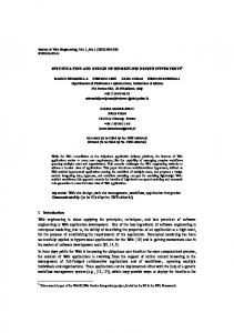


![Design and Implementation of a Workflow Engine - Sebastian Bergmann [PDF]](https://m.moam.info/img/260x300/design-and-implementation-of-a-workflow-engine-seb_647a109d098a9e35378b46a4.jpg)