Jun 17, 1999 - FILE CONTAINING NAMES AND TYPES OF GATES: C17.GAT . .... After a gate-level logic is synthesized from the register-transfer level (RTL) ...
TALLINN TECHNICAL UNIVERSITY
DESIGN ERROR DIAGNOSIS IN DIGITAL CIRCUITS BY
ARTUR JUTMAN
A Master Thesis Submitted to the Chair of Computer Engineering and Diagnostics of the Department of Computer Engineering
In fulfillment of the requirements for the Degree of Master of Science Computer Engineering
TALLINN June 1999
2
TABLE OF CONTENTS
1. INTRODUCTION .................................................................................................................................. 4 2. PRELIMINARIES .................................................................................................................................6 2.1 DESIGN AND VERIFICATION ................................................................................................................ 6 2.2 THE PROBLEM OF DESIGN ERROR DIAGNOSIS ..................................................................................... 7 2.2.1 Design Error Model .................................................................................................................... 8 2.2.2 Error Hypothesis ......................................................................................................................... 9 2.2.3 Ambiguity of Error Location ....................................................................................................... 9 2.2.4 Single and Multiple Design Errors............................................................................................ 10 2.2.5 Combinational and Sequential Circuits..................................................................................... 10 3. OVERVIEW OF DESIGN ERROR DIAGNOSIS METHODS....................................................... 12 3.1 WHAT MAKES A DESIGN ERROR DIAGNOSIS METHOD “GOOD” ....................................................... 12 3.2 A BRIEF CLASSIFICATION ................................................................................................................. 13 3.2.1 Simulation-Based Versus Symbolic Approaches ....................................................................... 13 3.2.2 Re-Synthesis Versus Error-Matching Rectification Approaches............................................... 13 3.2.3 Structure-Based Approaches ..................................................................................................... 14 3.2.4 Distinct Features of Sequential Circuit Oriented Approaches .................................................. 14 4. A NEW STUCK-AT FAULT MODEL ORIENTED METHOD ..................................................... 16 4.1 INTRODUCTION.................................................................................................................................. 16 4.2 DEFINITIONS AND TERMINOLOGY ..................................................................................................... 17 4.3 MAPPING STUCK-AT FAULTS INTO DESIGN ERROR MODEL .............................................................. 19 4.4 MACROS, PATHS, AND STUCK-AT FAULT MODELING ....................................................................... 21 4.5 FAULT TABLES AND VECTOR REPRESENTATION OF FAULTS ............................................................. 23 4.6 DESIGN ERROR DIAGNOSIS ALGORITHM ........................................................................................... 25 5. EXPERIMENTS................................................................................................................................... 29 5.1 PROGRAM DESCRIPTION .................................................................................................................... 29 5.2 RESULTS AND ANALYSIS OF EXPERIMENTS ....................................................................................... 31 5.3 CONCLUSIONS AND FUTURE WORK................................................................................................... 34 6. CONCLUSIONS................................................................................................................................... 35 7. REFERENCES ..................................................................................................................................... 36 APPENDIX A. DESIGN ERROR LOCALIZATION TOOL............................................................... 39 APPENDIX B. DIAGNOSTIC RESULTS FOR C17 ISCAS’85 BENCHMARK ..............................41 APPENDIX C. EXAMPLES OF FILES NEEDED TO RUN THE DIAGNOSTIC PROGRAM .....47 MACRO-LEVEL SSBDD MODEL FILE: C17.AGM ...................................................................................... 47 GATE-LEVEL SSBDD MODEL FILE: C17.GATE.AGM ................................................................................ 47 INPUT TEST PATTERNS FILE: C17.TST....................................................................................................... 48 SSBDD-NODE-TO-GATE-LEVEL-PATH RELATIONSHIP FILE: C17.PAT ...................................................... 49 FILE CONTAINING NAMES AND TYPES OF GATES: C17.GAT ...................................................................... 49
3
DIGITAALSKEEMIDE DISAINIVIGADE DIAGNOSTIKA Koostaja: Artur Jutman
ANNOTATSIOON
VLSI skeemide projekteerimine muutub iga aastaga üha keerukamaks seoses projektide mahukuse ja keerukuse kasvuga. Mida keerulisem on projekt, seda suurem tõenäolisus vigade tekkimiseks eri projekteerimise staadiumites. Algstaadiumides mitte avastatud vead võivad olla põhjuseks projekti maksumuse mitmekordistamises, projekteerimise aja märgatavas pikenemises ja valmistoodangu realiseerimise viivitamises. Antud asjaolud sunnivad teadlasi otsima ja välja töötama meetodeid projekteerimise vigade kiireks leidmiseks ja nende parandamiseks. Antud magistritöös on võetud vaatluse alla projekteerimise vigade diagnostika digitaalskeemides, on tehtud lühike analüüs olemasolevatest meetoditest ja on pakutud uus lähenemismeetod antud probleemi lahendamiseks. Juhendaja: Prof. Raimund Ubar
4
1. INTRODUCTION
Diagnostics finds place in many various aspects of our life. In medicine, for example, it is a human body condition determination. In industry it is a certain device condition determination. Such a device is called a unit under test. Diagnosis is a process of the unit under test analysis. The result of the diagnosis is a conclusion about the condition of the device. The conclusion can be, for example, one of the following: the device is working properly, the device is not working properly, and there is a defect in the device. Diagnosis is done in the field of digital electronics in order to discover defects in a digital system which could be caused either during manufacture or because of wear-out in the field. Testing for manufacturing defects is done at various stages in the production of a system: the dies are tested during fabrication, the packaged chips before placing in the boards, the boards after assembly, and the entire system is tested when complete. Testing for serviceability of a device is done during the whole lifetime of a device. The choice of test patterns for each of these tests is determined by factors such as the time available for test, the degree of access to internal circuitry, and the percentage of failures which are required to be detected. The theory and techniques of testing for manufacturing defects or operation faults are thoroughly studied in literature. The basics, for example, are given in [35, 36]. However, before the device is sent for manufacturing, it goes through many stages of design process. Each stage may be performed numerous times before an acceptable solution is obtained. The whole process is also iterative and may require circuit modifications in order to perform trade-offs. These modifications can be inserted either by means of automated designing tools or manually. For example netlists generated by the synthesis tools very often have to be modified by designers to improve timing performance, to obtain more compact structures, or to carry out small specification changes. The whole VLSI design process is getting more and more complicated due to continuously growing sizes and complexity of the projects. Due to this fact the error emergence probability through different design stages is big enough. An error not detected at the earlier stages may cause a cost explosion of the project and significantly increase the time-to-market. This fact forces the research in the direction of development fast and efficient methods for design error detection and rectification. The concept of design error slightly differs from one paper to another. In [5], for example, a design error is referred to an error in a specification but most authors treat the design error as an error in an implementation in relation to the specification. To avoid confusion, the latter concept is chosen in this work. An example of a design error could be a gate substitution error, for example, AND gate is replaced by OR gate in the implementation. It could be also a bad or missing connection between gates. Design error detection is usually performed at a validation phase using symbolic or simulation based design verification methods. Conventional verification tools can discover the functional difference between the specification and the implementation and provide counter examples in the form of input patterns that witness a difference between the implementation and the specification behaviors. Using these counter examples as input patterns, design engineers simulate the implementation to manually correct the
5
design. This process is called design error rectification. Here is where automatic methods may replace a lengthy manual correction saving a lot of debugging time. No matter what way of correction is applied the result must be verified again and the same diagnosis-correction-verification cycle is repeated until a correct design is obtained. There are several other applications of design error diagnosis techniques in fields that are closely related to the problem. For example, verification of a new version of design that is functionally equivalent to the previous one but has another timing or structure. Another one problem closely related to automatic error correction is engineering change [12]. It is called also incremental synthesis in [22, 23]. An old specification, an old implementation, and a new specification are given. . The goal is to create a new implementation fulfilling the new specification while reusing as much of the old implementation as possible. Suppose a specification of the design is slightly changed and a lot of engineering effort have already been invested (e.g., the layout of a chip may have been obtained). In this case it is desirable that such changes will not lead to a very different design allowing the reuse of the existing investment on the implementation. The quality of engineering change is measured by the amount of logic in the old implementation reused in the final new implementation. A couple of ideas how else the design error diagnosis can be used are given in [13]. The first one is a trick for logic minimization. The authors propose to inject intentionally two errors into an implementation and see if it can be corrected at just one location. The second application is debugging CAD tools that cause incorrect implementations. Software bugs existing in gate-level, timing, layout optimization, or technology mapping tools could be discovered diagnosing the incorrect implementation. The application domain of formal verification is no longer restricted to providing correctness of a specific design but it can also be used as a debugging tool and therefore helps speeding up the whole design cycle [2]. The next chapter of the thesis gives a general information about design error diagnosis issues and its location in a design process. A brief overview of existing approaches and requirements that make a design error diagnosis method good are presented in chapter 3. Chapter 4 describes a new approach for design error localization, based on stuck-at fault model. The program description and analysis of experiments based on this new method are presented in chapter 5. Finally, chapter 6 concludes the work.
6
2. PRELIMINARIES
Design of a digital system, as it was mentioned above, is a highly complicated process containing loops of repeating phases. Let us consider it in more detail and see where the design error diagnosis is located in the design process. We will also refine the problem of design error diagnosis in this section. 2.1 DESIGN AND VERIFICATION
Problem Definition System Requirements Specification System Partitioning Behavior
Process
Registertransfer
Modules
HW & SW Specifications
Logic
High-level Language
Design and Analysis
Physical
Object Code
Concept Development High-level Analysis
System Integration
Integration
Fig. 2.1 A top-down design process
The main stages of design process are shown in Fig. 2.1 according to [37] and [34]. The first step in any design process is to develop a description of a problem. For example, the problem may be to build a control system for an aircraft or a plant. The second step is to extract a set of requirements from problem description. They include typically cost, weight, size, power consumption, reliability, and so on. Then goes the system
7
partitioning step when the whole design is divided into set of smaller subsystems that can each be handled easily by individual teams of design engineers. During the concept development step several design approaches are considered and then analyzed in detail during high-level analysis step to find out advantages and disadvantages of one approach compared to another. Before the designers start the development of the final implementation, hardware (HW) and software (SW) specifications must be drawn up. The specifications must achieve a delicate balance necessary to meet system requirements and, at the same time, produce a practical, implementable, and manageable design. Then the design and analysis phase begins, when the HW and SW parts are concurrently developed. The analysis must be performed continuously during this phase to ensure that the system requirements are not compromised by design decisions that are made, and that hardware decisions do not negatively impact the software, and vice versa. The final step is the system integration, when all the subsystems, HW and SW parts are combined together and tested. If it is found that some element is not working properly in the system, then the design process for this element or several ones is repeated partly or completely. In order to achieve a reliable operation and a correspondence of device behavior to initial requirements with minimum costs, the design verification must be performed continuously in parallel to the design process. First of all, according to [37], the requirements design review must be applied to ensure that all necessary requirements have been identified, that they are reasonable and will be verifiable during the analysis and testing process. Then the conceptual design review occurs immediately after highlevel analysis step, to assure that the basic concept of a concrete candidate design is correct and meets the requirements that have been developed. During the specifications design review it is important to make sure that the specifications are both correct and understood correctly. Also, it is extremely important to guarantee that the designs will be testable. The detailed design review must encompass both the detailed design and the detailed analysis. Its purpose is to ensure that the specific designs meet the specifications and are capable of fulfilling the system requirements. The last checkpoint in the design process is the final review, the basic purpose of which is to examine the performance of the prototype and the results of the final analysis, to ensure that specifications have been adhered to and the system requirements have been met. If the design has been performed correctly and the design reviews have been successful throughout the design process, the final review should not uncover any major problems. On the right part of Fig. 2.1 the design and analysis stage of the design process is presented. The right part inside the oval belongs to a software design and the left one is a hardware design part. After a gate-level logic is synthesized from the register-transfer level (RTL) description it must be compared to the specification so that to detect any inconsistency. This is the exact point where the design error diagnosis is applied in order to find the erroneous area in the logic implementation. This procedure belongs to the most important and difficult part of the review process, the detailed design review. 2.2 THE PROBLEM OF DESIGN ERROR DIAGNOSIS Generally, the problem is defined as follows. Given a correct specification and an implementation. The goal is to find whether the implementation is correct or have errors inside. In the latter case, the task is also to localize the possibly minimum areas that contain the errors. In practice, gate level logic is treated as the implementation. The representation form of the specification varies from one approach to another. It could be
8
a description on either behavioral or RTL level or a graph representation of a circuit. Some structure-based approaches [5, 7, 9, 12] require also the information about structure of the “golden device” in the specification. We can try to check the physical level circuit for design errors by design error diagnosis technique too. For this purpose, we would turn everything upside-down. Suppose, we have the logic-level circuit checked for errors and found it to be correct. Then, we take the physical circuit as the specification and the logic as the implementation and apply a design error diagnosis method. If the implementation is proven to be incorrect, for example, AND gate should be somewhere instead of NOR gate, we can suppose that the NOR gate from the logic level has been improperly implemented in the physical level, where it is appears as the AND gate. If we know the exact place of the physical-level AND gate, the erroneous area could be then identified. 2.2.1 DESIGN ERROR MODEL Most of design error diagnosis methods rely on an error model. That means that in case of a certain behavior of a circuit, a certain type of error is suspected to be presented in it. In [20] a widely adopted simple design error model is proposed by Abadir et al. that includes following basic categories: ♦ functional errors of gate elements -
gate substitution
-
extra gate
-
missing gate
-
extra inverter
-
missing inverter
♦ connection errors of signal lines -
extra connection
-
missing connection
-
wrong connection
Gate substitution error means that a gate g is implemented by a wrong type of gate, for example, an AND gate is used instead a NOR. Simple extra gate means that two wires are accidentally gated together before feeding to another gate. Simple missing gate refers to the situation where a gate g is omitted and its inputs go straight to the place where its outputs should normally go (Fig. 2.2). g1
g5
& g3 g2
&
&
g4
&
g1
g5
& g3
g6
g2
&
&
&
b) Missing gate g4 Fig. 2.2 Missing gate example
g6
&
& a) Correct circuit
&
9
Extra/missing inverter means that an inverter is accidentally inserted/omitted on some line. Extra connection means that a wire is accidentally added from the output of a gate gi to the input of another gate gj. Missing connection refers to the reversed situation of extra connection. Wrong connection means incorrectly placed gate input. An input to some gate gk should have come from gate gi, but is mistakenly drawn from another gate gj. Gates in the model are restricted to primitive gates, i.e. AND, OR, NAND, NOR, XOR or XNOR, for simplicity. The disadvantages of using any error model are manifest when a real design error existing in implementation is not describable by the chosen model. However, in practice, the range of commonly encountered error types is limited. An experimental study described in [24, 25] has shown that the simple design error model covers about 98% of all the errors made by students. By the way, most frequently encountered error types were extra/missing inverter errors (Fig. 2.3). It is sensible then to start the diagnosis from inverter error verification continuing with all the others error types from the chosen error model in case the former has failed. �
�
�
�
�
�
�
�
�
�
�
�
�
�
�
�
�
&
$
'
�
(
/
0
1
1
0
2
/
0
1
1
0
)
�
�
�
�
�
�
�
�
�
�
�
�
�
�
�
!
"
#
�
$
4 2
5
6
�
7
8
)
%
)
*
+
,
�
+
-
.
,
0
)
*
+
,
)
*
+
,
2
.
3
+
Fig. 2.3 Distribution of design error classes [25]
2.2.2 ERROR HYPOTHESIS Error hypothesis is an assumption about an error(s) existing in an incorrect implementation. Error hypotheses are usually based on a concrete error model. In the case of the model described above, the error hypothesis may be any of the eight error types listed above. It could be also any combination of the errors, for example, a gate substitution and a missing inverter are supposed to be in the implementation. If the correction applied to the suspected erroneous area according to an error hypothesis fails, another hypothesis is usually chosen. 2.2.3 AMBIGUITY OF ERROR LOCATION Since there is more than one way to synthesize a given function, it is possible that there is more than one way to model the error in an incorrect implementation, i.e., the correction can be made at different locations. In Fig. 2.4(a), for example, a correct circuit is placed that occasionally was incorrectly implemented (Fig. 2.4(b)). We can correct the implementation either by changing back one OR gate to NAND, or another way, as shown in Fig. 2.4(c). The former correction based on a single gate substitution hypothesis, while the latter suppose both a gate substitution and a missing gate errors.
10
a b
(a ∨ b) & c & d
g1
1
g2
c
&
g1
a b
(a ∨ b) ∨ c ∨ d
1
g2
c
1
d
d
a) Correct circuit
b) Wrong implementation
a b c d
(a ∨ b) ∨ (c & d)
g1
1 &
g2 g3
1
c) Possible correction
Fig. 2.4 Multiple rectification possibilities
Another one example is given in [10]. In Fig. 2.5(a) a correct circuit is given. During logic synthesis process an extra OR gate was occasionally inserted (Fig. 2.5(b)). This error can be rectified using gate substitution hypothesis (Fig. 2.5(c)). Such examples for extra gate errors could be composed for any type of simple gates. The latter proofs that gate substitution hypothesis can also model simple extra gate errors, reducing the number of error types to check. More examples on error location ambiguity can be found in [13]. 1
&
& & a) Correct circuit
b) Wrong implementation
& c) Possible correction
Fig. 2.5 Gate substitution versus extra gate
All error hypotheses capable to rectify the circuit are considered equivalent. Error diagnosis methods are usually capable to find and correct an error within a functional equivalence class, which means that if a designer makes a simple design error, the error diagnosed is equivalent to that is made. This problem studied in more detail in [15] 2.2.4 SINGLE AND MULTIPLE DESIGN ERRORS The simplest scenario of design error localization appears in case when an implementation has only one design error from a chosen model. As there is only one error, the area of influence of the error is smaller than in case of multiple errors. Multiple errors, especially dispersed on a wide area of a circuit, may have influence upon a large part of the circuit and also upon each other. This makes it much harder to identify the exact locations of the errors and their types. However, as it was mentioned above, in some cases, occasionally inserted multiple errors could be rectified only at one place (Fig. 2.3(a)). And backwards, a single design error may be corrected by changing functions of several other gates (Fig. 2.3(c)). 2.2.5 COMBINATIONAL AND SEQUENTIAL CIRCUITS The diagnosis of combinational circuits is much easier than of sequential ones. As combinational circuits do not have memory and, therefore, do not retain information about previously applied test patterns, a choice of a test vector sequence does not affect the result of the test procedure; the diagnosis is based on an unordered set of diagnostic test patterns. On the contrary, when we deal with sequential circuits, instead of applying simple test vectors, we need to apply a specific sequence of vectors.
11
A sequential circuit can be seen as a succession of combinational ones over time frames. An error is repeated then in each copy of the combinational circuit. The added complexity is due to the fact that erroneous signals may have as sources not only the error location but also the present state for which the error effect has propagated from previous times. Thus, the error influence in a sequential circuit is growing from state to state that makes it harder to diagnose the circuit. However every sequential circuit is divided into a combinational part and a set of flipflops. This fact may give rise to the idea of testing a combinational part and flip-flops separately. The technique of testing a single flip-flop is trivial. It is needed to check the flip-flop truth table, that is all. The combinational part could be tested then as a conventional combinational circuit. However this strategy usually fails because the specification and the implementation may have different state encoding or even different number of states. This leads to the situation when one-to-one flip-flop correspondence between the implementation and the specification may not exist, and thus, the combinational approaches cannot be applied. A sequential error diagnosis approach is needed for this kind of situation.
12
3. OVERVIEW OF DESIGN ERROR DIAGNOSIS METHODS
In this chapter we will consider the previous work that is done in the field of design error diagnosis and describe several requirements for a “good” method. 3.1 WHAT MAKES A DESIGN ERROR DIAGNOSIS METHOD “GOOD” The problem of design error diagnosis is thoroughly studied in a past few years. Many different approaches and techniques have been developed this time. However this problem still remains a hot topic for researchers because of a strong demand from industry and drawbacks every known method have. Some of them are restricted to a certain type of errors they capable to diagnose, others are restricted to a circuit size or maybe require a lot of CPU time to solve the problem. In [15] several requirements are presented satisfaction of which allow a logic diagnosis technique to put into practical use: ♦ applicable to multiple design errors ♦ applicable to both gate errors and connection errors ♦ indicate error location(s) exactly: what gate(s) or what line(s) are erroneous ♦ provide detailed solutions for error rectification As the most frequent number of errors occasionally appeared during design process is 2 [24], a system not allowing the possibility of multiple error diagnosis has very restricted practical use. Several approaches also restrict an error model to only gate and inverter errors, however in [25] it is noted that the second of the most frequent appearing design error classes is wrong input wire error (Fig. 2.3). So, connection error diagnosis should be an essential part of a design error diagnosis system. The third requirement is not very clear because of discussed above ambiguity of error location. The sense of it should be understood as follows: the exact location of at least one of possible corrections must be provided. The best case is when the minimal possible change for the error correction is determined. The fourth requirement means that a diagnosis procedure should give not only information about what needs a correction but also how to correct it. We can add the speed requirement to this list. Large circuits may require a lot of time to diagnose an error. The faster the error is found the faster re-synthesis is performed the shorter the time-to-market. If a design process has many design cycles, any delay is multiplied with each cycle. Thus the method must be scalable to a circuit size. In other words, a perfect design error diagnosis method is a method providing the exact location of minimally possible change capable to correct the circuit. It does not rely on any error model to be able providing the correction for any possible design error. It is capable to find any combination of multiple design errors and does everything as fast as possible.
13
3.2 A BRIEF CLASSIFICATION We can classify available design error diagnosis and automatic rectification methods in many ways: combinational and sequential, simulation-based and symbolic, model-based or not, structure-based/not based, error-matching and re-synthesis, single and multiple error diagnosis approaches, and so on. Several years ago, most existing approaches relied on comparatively simple model-based single-error-matching techniques. On the contrary, most recent approaches are capable to find arbitrary errors due to their modelfree, multiple-error-oriented nature. 3.2.1 SIMULATION-BASED VERSUS SYMBOLIC APPROACHES Most error diagnosis approaches are either simulation-based or symbolic. The simulation-based approaches first derive a number of input vectors that can differentiate the implementation and the specification. These binary or 3-valued input vectors are called erroneous vectors or error detecting patterns. By simulating each erroneous vector, the potential error region can then be trimmed down gradually. The conditions for eliminating those signals that cannot be an error source vary from one approach to another. The symbolic approaches do not enumerate the erroneous vectors. They primarily rely on Ordered Binary Decision Diagram (OBDD) [21] to characterize the necessary and sufficient condition of a potential error source as a boolean formula. Based on this formulation, every potential error source can be precisely identified. In comparison, the symbolic approaches are accurate and extendible to multiple errors. However, constructing the required BDD representations may cause memory explosion when applied to large circuits. On the other hand, the simulation-based approaches, although scalable with the circuit size, are usually not accurate enough. ♦ simulation-based approaches [1, 3, 4, 6, 8, 10, 11, 14, 15, 16, 17, 18] ♦ symbolic approaches [2, 5, 12, 13, 19] ♦ mixed approaches [7, 9] 3.2.2 RE-SYNTHESIS VERSUS ERROR-MATCHING RECTIFICATION APPROACHES Rectification and diagnosis are slightly different notions. Diagnosis usually finds an error and rectification corrects it. Rectification methods mostly can be divided into three categories: ♦ re-synthesis based approaches [2, 3, 4, 5, 7, 9, 12, 19] ♦ error-matching based approaches -
single error approaches [6, 8, 10, 11, 13, 14, 16]
-
multiple error approaches [1, 15, 18]
Error-matching based approaches use an error model consisting of most commonly occurred types of errors. After error diagnosis, the implementation is rectified by matching the error with an error type in the model. This method is relatively restricted because, as it was mentioned above, it may fail when a real error in implementation can not be matched to any error in the model. Also, it is hard to be generalized for a circuit with multiple errors.
14
On the other hand, re-synthesis based approach is more general. These approaches rely on the symbolic error diagnosis techniques to find an internal signal in the implementation that satisfy the single fix condition, i.e., the condition of fixing entire implementation by changing the function of an internal signal. Once such a signal is found, a new function is realized to replace the old function of this signal to fix the error. In [12], a primary output partitioning algorithm was proposed to further enhance the capability of this approach. This enhancement makes it more suitable for solving engineering change problem. Theoretically this process will always succeed. But in the worst case, it may completely re-synthesize every primary output function. Another drawback of this approach is that it cannot handle larger designs because of using OBDD. 3.2.3 STRUCTURE-BASED APPROACHES Structural approaches [5, 7, 9, 12] mostly rely on finding structural similarities between a specification and an implementation. This has been shown to be effective in reducing the verification complexity of large combinational circuits [9,23]. These approaches require a structural description for the specification or reference circuit. First, equivalent signal pairs in two circuits are identified. The more the similarity degree between the two circuits, the smaller the part of implementation remained for further diagnosis. The technique applied then, to search error(s) in this remained area, may be various. In [24], for example, a heuristic called back-substitution is employed in hopes of fixing the error incrementally. In [5] a symbolic re-synthesis approach is used. The major drawback of structural approaches is that the success of the whole procedure is highly depended on existence of structural similarity between two circuits. However, these approaches could be suitable for large circuits. 3.2.4 DISTINCT FEATURES OF SEQUENTIAL CIRCUIT ORIENTED APPROACHES Due to special features of sequential circuits, combinational approaches could not be directly applied to them. However, with certain modifications done, some simulationbased combinational circuit oriented approaches can be used for sequential circuits too [11, 3]. In [11] a modified combinational circuit approach is presented that is based on the method presented in [10]. The authors introduce a concept of Possible Next States that are the set of states reachable from a given initial state, or set of initial states, due to the existence of several possible locations of the error. The implementation of the sequential circuit is represented by its iterative logic array model. The circuit is then simulated in each time frame separately, and diagnosed by applying combinational diagnosis rules, where the present-state lines are treated as primary inputs, and the nextstate lines as primary outputs. Before proceeding to the analysis in the next time frame, the set of possible next states is computed, and then the analysis is done in the next time frame under the application of each one of these possible next states. This operation is repeated until the error is found. A drawback of this approach is that they consider registers and flip/flops as basic components of the circuit description and the diagnosis is only concerns the combinational part of the circuit. This method also relies on a restricted error model and could not rectify multiple errors. Some sequential approaches also use symbolic techniques [7]. In these approaches, the circuits are regarded as finite state machines (FSM) and characterized by a transition relation and a set of output functions using BDD's. A product machine is constructed and its state space is traversed. Most of them assume a reset state, and employ a
15
breadth-first traversal algorithm to compute the set of reachable states. The equivalence of these two machines can be proved by checking the tautology of every primary output of the product machine. Due to the memory explosion problem, these approaches can easily fail for large designs. In [7] a hybrid approach is presented that combines symbolic BDD techniques and exploiting structural similarity between two circuits. The key idea in these algorithms is that, instead of directly examining the functional equivalence of the primary outputs, equivalent flip-flop pairs and equivalent internal signal pairs are first identified. This process proceeds forward from the primary inputs towards the primary outputs. Once an internal equivalent signal pair is identified, it is merged to speed up the subsequent verification process. This approach can show good results if the two circuits are structurally similar. This approach can be also less vulnerable to memory explosion problem.
16
4. A NEW STUCK-AT FAULT MODEL ORIENTED METHOD
4.1 INTRODUCTION In [26] and [27] general ideas and basic theoretical concepts for a new hierarchical design error diagnosis method are presented. The method is based on the stuck-at fault model, where all the analysis and reasoning is carried out in terms of stuck-at faults and only in the end, the result of diagnosis will be mapped into the design error area. Such a treatment allows exploiting traditional ATPGs to serve the problem of design error diagnosis. Another distinct feature of the method is that it uses a new model of structurally synthesized BDDs (SSBDD) [32]. In contrast to BDD or OBDD circuit representations the complexity of SSBDD representation model generation does not grow exponentially with the circuit size but only linearly [32]. In addition SSBDD representation preserves structural information about circuit allowing developing fault diagnosis procedures that are more efficient for increasing the speed in error detection and localization that gatelevel ones. On SSBDDs, a primary set of suspected faulty signal paths are calculated. Based on these paths, a list of suspected erroneous gates is generated, which subsequently will be reduced to the minimum by using the information obtained from the test experiment. Our approach combines both verification and error localization techniques together. The information gathered on the verification stage is used then during localization reducing the time needed for the whole process. Due to the facts enumerated above, our method provides one of the fastest erroneous area localization processes among other known methods. Another advantage of the method is that it is not structure based. In other words, the specification can be represented on any level of abstraction; it can be given as a truth table, as a BDD, as another gate-level circuit, or in form of Boolean formula. We use SSBDDs only to represent the erroneous implementation. They can be generated directly from gate-level netlists. Thus, the success of our method does not depend on any structural similarity between the specification and the implementation. Although, our method is based on a restricted to gate-substitution and inverter errors simple error model of Abadir et al. [20], it was shown above that simple extra gate errors could be rectified using only gate substitution error model. So, missing gate error and connection types of errors are remained out of the scope of this work. They, as well as multiple errors, are the subject of our future work. The work described in this chapter represents the implementation of the method. Refined fault calculation procedure is developed and described in detail. The presented material has been also accepted for publication [28, 29].
17
4.2 DEFINITIONS AND TERMINOLOGY Consider a circuit specification, and its implementation. The way of representation for the specification is not significant. Only relationship between input patterns and output responses in specification is important. However, without loss of generality, let the specification and the implementation are given at the Boolean level. The specification output is given by a set of variables W = {w1 , w2 , ... , wm}, and the implementation output is given by a set of variables Y = {y1 , y2 , ... , ym}, where m is the number of outputs. Let X = {x1, x2, ... , xn} be a set of input variables. The implementation is a gate network and Z is a set of internal variables used for connection of gates. Let S be the set of variables in the implementation S = Y ∪ Z ∪ X. The gates implement simple Boolean functions AND, NAND, OR, NOR, XOR, XNOR and NOT. An additional gate type FAN is added (one input, two or more outputs) to model fanout points (Fig. 4.1). It is not used in the diagnostic procedure but needed in several definitions below. Fanout point & &
FAN & FAN gate
Fig. 4.1 A FAN gate
We use two different levels for representing the implementation: gate and macro-level representations. Let XF and ZF be the subsets of inputs and internal variables that fanout (they are input to a FAN gate). Let ZFG be the subset of internal variables that are output of a FAN gate. At the gate level, the network is described by a set NG = {gk} of gate functions sk = gk (sk1, sk2, ... ,skh) where sk ∈Y ∪ Z, and skj ∈ (Z - ZF) ∪ (X - XF). At the macro-level, the network is given by a set NF={fk} of macro functions sk = fk(sk1, sk2, ..., skp) in an equivalent parenthesis form (EPF) [31], where sk ∈Y ∪ ZF, and Sk = {sk1, sk2, ..., skp}⊆ZFG ∪ (X - XF) be its set of inputs. In other words, a macro is a tree-structured subcircuit with no fanout points inside. It has several inputs and only one output (Fig. 4.2). &
& A macro function
& &
& &
Fig. 4.2 An example of a macro function
18
The following design error types are considered throughout the paper in relation to gates gk ∈NG. Definition 1. Gate replacement error. It denotes a design error which can be corrected by replacing the gate gi in NG with another gate gj , by gi → gj. The “→” sign refers to “is replaced by”. Definition 2. Extra/missing inverter error. It denotes a design error which can be corrected by removing/inserting an inverter at some input s ∈ X, or at some fanout branch s ∈ ZFG : s → NOT(s). Definition 3. Single error hypothesis. Our design error diagnosis methodology is based on a single error hypothesis where it is assumed that in the circuit a single error from the following error types can exist: 1) an extra/missing inverter, 2) a random gate replacement between AND, OR, NAND, NOR, XOR and XNOR gates. From these definitions it should be clear that only inverters occasionally inserted/omitted at a gate input or at a primary input of a circuit are treated as extra/missing inverters. The inverters inserted/omitted at a gate output are covered by gate replacement error type (Fig. 4.3).
Extra inverter error
NAND → AND error
1 &
1
&
Fig. 4.3 Extra inverter and gate replacement errors
Definition 4. Test patterns. For a circuit with n inputs, a test pattern T'i is a n-bit vector which may be binary Bn or ternary Tn, where B = {0,1} - the Boolean domain, T = {0,1,U} - the ternary domain, where U - is a don’t care. Denote the set of all test patterns applied to a circuit during one test experiment as T = {T1, T2, ... Tt}, where t is a number of test patterns. Definition 5. Stuck-at fault set. Let F be the set of stuck-at faults s/1 and s/0, where s∈Z∪X. Definition 6. Detectable stuck-at faults. A test pattern Ti detects a stuck-at-e fault s/e, e∈{0,1} at the output yj, if when applying the test pattern Ti to the implementation and the specification, the result yj(Ti) ≠ wj (Ti) is observed. Let us call s/e a detectable by a test pattern Ti at the yj output stuck-at fault. Denote the detection information as ε(Ti, yj), where 9
:
;
i
and as δ (Ti, yj), where
0, if the test Ti passed at y j , y j ) = 1, î if the test Ti detected an error at y j
19
0, stuck - at 0 (s/0) is detectable by T at y i j δ(Ti , y j ) = 1, stuck - at 1 (s/1) is detectable by Ti at y j X, no fault is detectable by T at y i j î Denote a set of stuck-at faults detectable by a test pattern Ti at an output yj as F(Ti, yj), then let F(Ti) =
F(Ti , y j )