Design, Modeling, and Simulation of the Modular Distributed

Design, Modeling, and Simulation of the Modular Distributed Manipulator System Jonathan E. Luntz, William Messner, and Howie Choset

Contents

1 Introduction

1

2 Prior Work 3 Modeling

4 5

1.1 Prototype System . . . . . . . . . . . . . . . . . . . . . . . . . . . . . . . . . . . . . . . . . . . . . . 1.2 Operation and Modeling of Actuator Arrays . . . . . . . . . . . . . . . . . . . . . . . . . . . . . . .

3.1 3.2 3.3 3.4 3.5

Wheel-Object Interaction Supporting Forces . . . . Translational Dynamics . Rotational Dynamics . . . Other Friction Modes . . 3.5.1 Coulomb Friction . 3.5.2 No-Slip Friction . .

. . . . . . .

. . . . . . .

. . . . . . .

. . . . . . .

. . . . . . .

. . . . . . .

. . . . . . .

. . . . . . .

. . . . . . .

. . . . . . .

. . . . . . .

. . . . . . .

. . . . . . .

. . . . . . .

. . . . . . .

. . . . . . .

. . . . . . .

. . . . . . .

. . . . . . .

. . . . . . .

. . . . . . .

. . . . . . .

. . . . . . .

. . . . . . .

. . . . . . .

. . . . . . .

. . . . . . .

. . . . . . .

. . . . . . .

. . . . . . .

. . . . . . .

. . . . . . .

. . . . . . .

. . . . . . .

. . . . . . .

. . . . . . .

. . . . . . .

. . . . . . .

. . . . . . .

. . . . . . .

. . . . . . .

2 4

6 7 9 10 12 12 12

4 Simulation

13

5 Discussion A Appendix: Derivations of Other Friction Modes

17 19

4.1 Simulation Model . . . . . . . . . . . . . . . . . . . . . . . . . . . . . . . . . . . . . . . . . . . . . . 13 4.2 Simulation Results . . . . . . . . . . . . . . . . . . . . . . . . . . . . . . . . . . . . . . . . . . . . . 16

A.1 Coulomb Friction . . . . . . . . . . . . . . . . . . . . . . . . . . . . . . . . . . . . . . . . . . . . . . 19 A.2 No-Slip Friction . . . . . . . . . . . . . . . . . . . . . . . . . . . . . . . . . . . . . . . . . . . . . . . 20

1 Introduction Distributed manipulation is the method of inducing motion on an object through the application of many external forces. An actuator array is a form of distributed manipulation where many small stationary elements (which we call cells) cooperate to manipulate larger objects. In such systems, an object lies on a regular array of cells. Many cells support the object simultaneously, and as it moves, the set of supporting cells changes. While supporting the object, each cell is capable of providing a traction force on it, and the combined action of all the cells supporting the object determines the motion of the object. Through proper coordination, the array translates and rotates objects which ride on top of the array. Since actuation is distributed, each of many parcels can be manipulated independently, appearing as if each parcel were carried separately by a mobile vehicle (Figure 1). 1

Figure 1: The MDMS: Several parcels can be translated and rotated, independently.

Figure 3: A prototype cell made up of a motorized pair of roller wheels mounted orthogonally.

Figure 2: A roller wheel which allows free motion along its axis of rotation.

Current applications of actuator arrays include microelectromechanical systems transporting pieces of silicon wafer and large-scale arrays of motorized wheels transporint cardboard boxes. The Modular Distributed Manipulator System (MDMS) is such a large-scale actuator array.

1.1 Prototype System

We have built a prototype MDMS in which each cell each cell consists of a pair of orthogonally mounted motorized roller wheels (Figures 2 and 3). These wheels are capable of producing a force perpendicular to their axes, while allowing free motion parallel to their axes. The combined action of the two roller wheels is to eect force in any planar direction to an object resting on top of the array. Each of these cells is connected to a large breadboard style base (Figure 4) to create a regular array of manipulators. Currently, we have 18 cells which can be arranged arbitrarily in a 2-D grid. A photograph of the prototype MDMS is shown in Figure 5. Each cell is controlled by an inexpensive single-board computer based on the MC68HC11 microcontroller. We are exploring the use of distributed control on the MDMS because it is a relatively underdeveloped and interesting control paradigm, and because we believe that it would become impractical or impossible for a single computer to control hundreds or possibly thousands of cells. Each cell communicates with its four neighboring cells, allowing messages to be passed along the array. In addition, each cell contains one (or more) binary sensors to detect the presence of an object. Figure 6 shows this control architecture. For many applications, a dedicated robot or conveyor belt is the simplest and most appropriate solution. There are cases, however, where features provided by the MDMS, such as exibility, modularity, redundancy, and 2

Figure 4: Two-dimensional array of cells arranged in a grid.

Figure 5: Current experimental setup. A cardboard box rests on top.

Figure 6: A few manipulator cells carrying a parcel. Neighboring cells can communicate.

3

recon gurability, are required. The MDMS can be used in conjunction with traditional robots and conveyor belts to form hybrid systems. For example, in airport baggage handling, long conveyors can be used to transport bags over long distances while MDMS arrays can be installed at conveyor junctions to sort and to re-direct baggage trac. In exible manufacturing, the MDMS can be used to transport objects between robot workspaces where simple robots are used for object xturing.

1.2 Operation and Modeling of Actuator Arrays

To use an actuator array for object manipulation, two modes of operation may be used: open-loop (passive) and closed-loop (active). In a passive mode, the action of the cells is pre-programmed and constant, and a \force eld" is established in which the object moves. In an active mode, the array uses information about the object's motion to update the action of the cells. Local sensors at each cell or some global sensor, such as a vision system, provide such information, and in either case, real-time communication either to or between cells is generally necessary. Passive modes are useful for object positioning and orientation tasks with simple maneuvers which do not require extreme precision. Active modes are generally useful for more precise motions or more complex motions involving multiple objects. It is usually simpler and less expensive to implement an open-loop mode since no feedback or control is necessary. For an open-loop system, it is generally desirable to scale the actuator array so that very large numbers of cells support an object. This provides an approximately continuous medium on which the object can rest, resulting in smoother and more predictable motion. In the limit of very small cells placed closely together, the array does in fact become a continuous medium providing a true force eld. In certain cases, the motion of an object on such a eld is analytically predictable. If the force eld is designed to be conservative, potential eld theory applies[5]. Unfortunately, it is usually impractical to construct a system with enough actuators to justify the continuous medium approximation. The manipulated objects must be supported by relatively smaller numbers of cells. This requires that the discrete nature of an actuator array be taken into account when designing open-loop elds and when predicting the motion of objects. Therefore, for full functionality of the MDMS, and actuator arrays in general, a thorough understanding of the dynamics of object manipulation on a discrete array is necessary. Such an understanding enables the design of static force and velocity elds and the design of active manipulation strategies to transport and manipulate objects arbitrarily. To design both open-loop and closed-loop control schemes we must be able to predict the motion of an object on the actuator array. This requires an understanding of the dynamics of manipulation on the actuator array. A relationship between the control inputs (in our case, the speeds of the wheels) and the net forces and motion of the object must be established. The purpose of this paper is to examine these dynamics of manipulation on the MDMS and other discrete actuator arrays. The net force and moment acting on the object as a function of the object's position, orientation, current motion, and set of supports are derived. An understanding of the open-loop dynamics, where wheel speeds are held constant, is required to design closed-loop control schemes. Therefore, this paper focuses on the open-loop case. Section 2 brie y describes some prior work done in actuator arrays by the authors and by other researchers. The dynamics of object manipulation on the MDMS are examined in Section 3, where the dynamics of manipulation are analyzed using a spatially discrete representation of the forces in the system. A simulator is presented in Section 4 which exploits some of the dynamic properties of the system to improve eciency. Several test cases are simulated. The results of the paper are discussed in Section 5.

2 Prior Work The use of open-loop elds for object manipulation originally stemmed from ideas in minimalistic manipulation. Mason and Erdmann [1, 3] provided a radical alternative to standard robotic manipulation by signi cantly simplifying the robot manipulator and developing manipulation algorithms for these low-degree-of-freedom sensorless 4

mechanisms. Goldberg [4] developed an algorithm which orients an object with a sequence of gripper open, close, and rotation operations without sensor information. This sequence of operations is termed a squeeze. Bohringer, et. al. [2] applied this type of sensorless manipulation to an array of micromechanical actuators which were used to manipulate very small objects. They analyzed a \squeeze" eld which has a similar action to a gripper squeeze on an object. Their analysis used a continuous eld approximation and assumed that the net eect of the actuators was to apply a constant force per unit area on the object. They showed that squeezed elds manipulated polygonal objects to one of a nite number of orientations. Kavraki [5] supplied further analysis of microactuated systems using elliptical potential elds to orient objects to a single orientation with a single eld. Potential functions are used to predict stable con gurations of objects. Continuous potential functions adequately approximate Kavraki's and Bohringer's systems, because many microsized cells support a larger object. The MDMS, on the other hand, requires the explicit modeling of the discrete forces in the system. The authors rst began to model the discrete dynamics of manipulation in one dimension along a single row of cells[6] where it was rst found that the parcel experiences piecewise constant linear dynamics as it moves along the array. In this work (and the other work leading up to this paper), the discrete nature of the system was modeled explicitly, taking into account the distribution of weight of the object amongst the cells and the speci c interaction between each wheel and the object. That work was extended into two dimensions (plus rotation) in a following paper[7] which is a precursor to the work presented here. Much of the modeling in its nal form presented here is presented in another precursor paper[9]. The authors presented work on modeling nonlinear friction modes, including mixed stick-slip friction modes in another paper[8] along with a rudimentary simulator. The simulator presented here is much more ecient since it takes advantage of the piecewise nature of the dynamics. In addition to the dynamics of manipulation on the MDMS, the authors have examined other practical and dynamic issues of the MDMS. Further details on the MDMS prototype as well as simple tests of the system's functionality can be found in previous papers by the authors [10, 12]. The authors have developed and tested a distributed network and a communications language for the ecient passing of messages between the cells [13]. Another aspect of the dynamics of the MDMS was examined in the paper where the system (then referred to as the Virtual Vehicle) was rst introduced[11]. In that paper, the distributed dynamics of the wheels, without an object on top, was examined. It was found that under a simple communication protocol between neighboring cells, the overall spatial dynamics of wheel speeds had the form of the discretized transient heat conduction equation with wheel speed analogous to temperature. This lead to the idea that physical analogies such as heat transfer, electric elds, and uid ow could be used to design potentiallly useful behaviors on a system with distributed dynamics and control. While these other issues are interesting and important in the implementation of the MDMS, they are secondary to understanding the dynamics of object manipulation, and are not discussed further in this paper. This paper presents the dynamics of manipulation in two dimensions plus rotation under one of several models of friction between te wheels and the object.

3 Modeling In this paper, we are interested in computing the net force and moment acting on an object as it moves along the MDMS array. The force and moment are functions of the position of the object, the speed at which the objet is moving, the set of cells supporting the object, and the speeds of the wheels in those cells. The basic approach in the paper is to examine the situation where the object rests on a particular arbitrary set of cells, compute the forces as a function of object position and motion, and then recompute if the set of supporting cells changes. First, we discuss the interaction between the wheels and the object, and then we compute the forces acting on the object. The following assumptions will be made: 5

    

Each orthogonally oriented pair of wheels acts as a single support. Supports act as springs to support the parcel. The bottom of the parcel is at. The speed of each wheel is constant. Horizontal force between each wheel and the parcel is due to sliding friction, and relative motion always exists between the obejct and each wheel (except in one case, where it is assumed that no relative motion exists between the object and any of the wheels).  The friction is modeled by one of several simple laws duscussed later. To compute the horizontal translation and rotation dynamics of the parcel, rst we use the vertical equilibrium of the parcel and constitutive relations for the supports to compute the normal forces supporting the parcel. Then we apply a friction model between the parcel and wheels is to determine the traction force from each cell. These traction forces are summed over all cells supporting the object, and the net force and torque acting on the object are functions of the object's position and motion. The structure of the mathematics and several convenient mathematical identities simpli es the problem considerably.

Notation: Because of the large number of variables used, this paper will employ a consistent notation. Scalar variables will appear in normal math font (e.g. s), vectors will appear in normal math font with an arrow (e.g. ~v ), and matrices will appear in bold font (e.g. m). Subscripts x and y will indicate x and y components, and subscript

will indicate the ith cell. Vectors with x and y components are generally column vectors, and vectors with a component for each cell are generally row vectors. Variables with both x and y components and components for each cell are represented as matrices. For example, V is a matrix made up of velocity (column) vectors V~i for each cell, with components Vxi and Vyi . V can also be said to be made up of component (row) vectors V~x and V~y listing the velocity components for all the cells.

i

3.1 Wheel-Object Interaction

A model of the contact between the wheels and object riding on the array is essential for modeling the dynamics of object manipulation on the MDMS. In the model, each wheel applies a force in the plane to the object through friction between the wheel and the object as shown in Figure 7. There are several possible models of this friction force.

Viscous Friction. The wheel slides on the object. The friction force is proportional to the normal force between

the wheel and the object and the dierence between the wheel's speed and the speed (in the direction of the wheel) of the surface of the object at the wheel. The roller wheels used in the prototype system ensure that the friction will only occur in the direction perpendicular to the wheel's axis. The assumption is that the motor is strong enough to maintain its speed regardless of the traction force. Coulomb Friction. The wheel slides on the object. The friction force is proportional to the normal force between the wheel and the object. The direction of the friction will be the same as that in the viscous case. The assumption is that the motor is strong enough to maintain relative motion between the wheel and the object. No-Slip Friction. The wheel rolls on the object. The traction force is not a function of the normal force, and there is no relative motion (in the direction perpendicular to the wheel's axis) between the wheel and the object. The wheel rotates to follow the motion of the object, and the traction force depends on the properties of the motor and the voltage applied to the motor. 6

Ni

Xcm fi

Vi

Figure 7: Interaction between wheel and parcel. The rotating wheel supports the object and provides a traction force. We will examine the dynamics of the object mainly under a viscous friction model, since this most closely matches the observed qualitative behavior of the prototype system. We will discuss the eects of the other friction models. Since the sliding friction modes (viscous and coulomb) depend on the normal force, we must rst compute the normal forces as a function of the object's position. This is the topic of the next section.

3.2 Supporting Forces

Consider the case where n cells support an object. Approximating the two-wheel support of each cell as a single point support, we need to solve for n forces supporting the object. These n point supports are arranged arbitrarily in the x-y plane having coordinates as entries of the matrix below.

X=

~x x y ~

=

1 : : : xn

y1 : : : y n

  = X~

~ 1 : : : Xn



(1)





An object, whose center of mass is located at X~ cm = xcm ycm T resting on n of these cells, is supported by vertical normal forces   ~ = N1 : : : Nn : (2) N The object must be in equilibrium in the vertical direction and in rotation about the x and y axes. The vertical equilibrium of the object, with weight W , requires that n X i=1

Ni



=W = 1

:::

1

 N~ T:

(3)

Rotational equilibrium about the x and y axes require that the moments induced by the normal forces about any point (in this case, the arbitrarily located origin of our coordinate system) sum to the moment about this point induced by the weight of the object. The moment equilibrium about the x and y axes, respectively, requires that n X

i=1 n X i=1

Ni yi

= ~y N~ T = W ycm ; and

(4)

Ni xi

= ~x N~ T = W xcm :

(5)

At this point in the development, there are n unknowns (the elements of N~ ), but only three equations (3,4, and 5) from equilibrium. To solve for the remaining n ? 3 forces, we must consider exibility in the system. A simple physical model of this exibility is shown in side view in Figure 8. Each support is assumed to be a spring, with Hooke's Law (Ni = Ks
zi ) representing the compression of the ith cell under a normal load. Physically, this 7

Figure 8: Flexible supports in many-cell case.

exibility can be thought of as a exible suspension under each wheel, such as the next generation of our hardware array will include. In the current system, an equivalent exibility is apparent in the bottom of the object, either in the cardboard of a box, or a foam pad on which the box rests. Assuming the bottom of the box is nominally at, the exible cells conform to the bottom of the box to distribute the weight. All the cells (under the object) lie in this plane. A representation of the plane of the bottom of the object is z = a0 y + b0 x + c 0 : (6) Each cell will obey the following displacement relation: a 0 y i + b 0 xi

+ c0 ayi + bxi + c = 0


zi = Ni =Ks = ) Ni +

(7)

Equations 3, 4, and 5 along with n instances of Equation 7 supply n + 3 equations and n + 3 unknowns (n Ni 's and 3 plane parameters, a, b, and c). The matrix form of this system of equations is

2 1 66 ... 66 0 66 64 1 x1 | y1

0 1 x1 y1 . . . .. .. .. .. . . . . : : : 1 1 xn yn ::: 1 0 0 0 : : : xn 0 0 0 : : : yn 0 0 0 {z A :::

32 N 77 66 ...1 77 66 N 77 66 n 75 64 c b a } | {z

T N~ abc

3 2 0 77 66 ... 77 66 0 77 = 66 75 64 W W xc } | W{zyc W~

3 77 77 77 : 75 }

(8)

The top portion of this equation represents the n instances of the compatibility equation (Equation 7). The bottom three rows represent the vertical, x-moment, and y-moment equations (Equations 3, 4, and 5). This equation can be inverted to solve for N~ abc (which contains N~ and a, b, and c.) ~T N abc

~ = A?1 W

(9)

Since A is symmetric and very structured, its inverse is easy to compute. De ne the matrix B as

2 1 B = 4 x1 y1

::: ::: :::

8

1

xn yn

3 5:

(10)

The block form of the matrix A is

  T (11) A = InBn 0B33 : The inverse of the matrix A exists if B has rank 3. B has rank 3 if and only if all the cells under the object are not co-linear. The expression for the inverse is

"

?BBT
?1 B BT ?BBT
?1# ?
: ? BBT ?1 BBT
?1 B

T A?1= Inn ?? B

(12)

(The reader is invited to verify the form of the inverse by multiplying A by A?1 .) ~ only multiplies nonzero elements into the right side of A?1 , and only the slopes (a, b, and c) result Since W from the lower portion of A?1 , only the upper right partition of A?1 is used to calculate N~ . The expression for ~ is N

2 W 3
? ? 1 ~ T = BT BBT 4 W ycm 5 N 0W2ycm1 3 2 0 ?
= W BT BBT ?1 @4 0 5+4 1 0

0 0 0 1

3 1 5 X~ cmA :

(13)

Note that there are cases where one or more of the normal forces in N~ will be negative. Since the object cannot actually \pull" on the springs in the support model, the normal forces must be recalculated with the negative supports removed from the set of supports.

3.3 Translational Dynamics

We will now represent the planar dynamics of an object resting on the array as a net planar force and torque acting on the object as a function of the object's position, linear velocity and rotational velocity. We will rst apply the viscous friction model to derive the planar forces from the supporting forces as shown in Figure 7. Under the viscous friction assumption, the horizontal force from each cell f~i is proportional to a coecient of friction , the normal force Ni exerted by the cell, and the vector dierence between the velocity of the wheel and the velocity of the parcel at the point of the cell. This velocity dierence is a function of both the translational velocity of the parcel, X~_ cm , the velocity of the wheel, V~i , the rotation speed of the parcel about its center of mass, ~i ? X ~ cm . ! , and the position dierence between the cell and the center of mass, X f~i



=  V~i

?

~_ cm + ! X



0 1 ?1 0



~i X

?

~ cm X



Ni

(14)

The total horizontal force is the sum of the f~i over all the cells. To simplify notation, the wheel velocity matrix, V, is de ned.   (15) V = VV1x VV2x :: :: :: VVnx 1y

2y

ny

Inner product notation eliminates the explicit summation, and the expression for the net horizontal force vector is f~

=

n X ~ i=1

fi

   =  V ? X~_ cm 1 1 : : : 1 9



+! ?10 01





 ~ T



X ? X~ cm1 1 : : : 1

N

  = V N~ T ? X~_ cm 1 1 : : : 1 N~ T      +! ?10 01 X N~ T ? X~ cm 1 1 : : : 1 N~ T :

(16)

Note that 1 1 : : : 1 N~ T is the sum of the normal forces, which is the parcel weight, W . Therefore, the last two terms in the parentheses are identically zero from Equations 4 and 5. Hence, the net horizontal force is not a function of the parcel's rotation speed and Equation 16 becomes ~ T ? X ~_ cm W: f~ = V N (17) The second term in Equation 17 is a linear damping term, which is always dissipative, since weight is positive. The result of substituting N~ from Equation 13 into Equation 17 is

20
? ?1 4 1 f~ = W VBT BBT

3 5 X~ cm | {z } k 213 ?
+ W VBT BBT ?1 4 0 5 ?X~_ cm W 0 | {z } 0 0 0 1

s

f~o

= ks X~ cm + f~o ? W X~_ cm ;

(18)

where ks is a constant 2  2 matrix and f~o is a constant 2  1 vector. The matrix ks is essentially a matrix of spring constants, since it speci es force as a linear function of position. The vector f~o is an oset force. The translational dynamics of the object are piecewise constant and linear (as the object changes supports). Therefore, it is easy to predict the local translational motion of the object.

3.4 Rotational Dynamics

In two dimensions, the torque each cell applies to the parcel is the scalar cross product of the position vector of the point of application of the force, X~ i , relative to the parcel center of mass, X~ cm, and the horizontal force vector from that point, f~i . Applying the matrix de nition of scalar cross products, and taking f~i from Equation 14 (viscous friction), the ith cell applies the following torque, i :



  ~ ~ Xi?Xcm Ni ?  ?   = X~ iV~i Ni ?X~ cmV~i Ni ? X~ i?X~ cm X~_ cm Ni ~ ~ T 0 1  0 1 ~ ~  ~

~ cm i =  Xi X

+!

?

 ~

Xi Xcm

~_ cm + ! Vi X

0 1 ?1 0

?1 0 ?1 0

?

Xi Xcm Ni

(19)

To simplify notation de ne Ri = X~ iV~i , which de nes the components of the vector R~ , and Xi = X~ iT X~ i , which de nes the components of the vector X~ . The product of cross product matrices is ?I22 . In addition, use the fact 10

T X ~ i , and that reversing the order of a cross product changes sign, to obtain that X~ iT X~ cm = X~ cm ~ ~  ~ cmV ~i Ni +  X ~_ cm X i = Ri Ni ?X i?Xcm Ni

~

?!

=

?

~ cm Xi X

T  ~



?

~ cm Ni Xi X

~ cm V ~i Ni +  X ~_ cm Ri Ni X





?   X~ i?X~ cm Ni     T ~ ~T X ~ i?X ~ cm Ni : ?! Xi Ni?X~ cm Xi Ni?X cm





T 

(20)

Note that the term multiplying ! is positive since Ni and the product X~ i?X~ cm X~ i?X~ cm are always positive. The total torque is the sum of the i over all the cells. Inner product notation eliminates the explicit summation, and the expression fot the total torque is 

=

X

i

= R~ N~ T ?X~ cmVN~ T     +X~_ cm XN~ T?X~ cm 1 1 : : : 1 N~ T





T ?! X~ N~ T?X~ cm XN~ T   ~T ~  T XN ?Xcm 1 1 : : : 1N~ T : ?X~ cm



(21)

~ cm , and 1 1 : : : 1 N ~ = W from parcel equilibrium (Equations 3, 4, and 5), Since XN~ = W X  XN~ ?X~ cm 1 1 : : : 1 N~ = 0 and the expression for torque reduces to 



T ~ = R~ N~ ? X~ cmVN~ ? ! X~ N~ ?W X~ cm Xcm



(22)

:

The last term in this expression is ?! multiplied by a positive term (from Equation 20) and hence is dissipative. Substituting the expression for normal forces from Equation 13 into Equation 22 results in an expression for the moments acting on the parcel as a function of position and rotational speed. 213
? ? 1 ~ BT BBT 405  = W R 0

|

{z

} 20 03 ?
? 1 T T 41 05 X~ cm + W R~ B BB 01 {z } | ~k     T X ~ cm +X~ cm f~o+ks X~ cm ?! X~ N~ ?W X~ cm  ~ ~ ~ ~ ~ ~ ~ o

s



T X ~ cm = o + ks Xcm ? fo + ks Xcm  Xcm?! X N?W X~ cm

(23)

where ks and f~o are the spring and oset constants from the translational dynamics (Equation 18), ~ks is a 1  2 constant vector relating torque to position, and o is a scalar constant torque. Note that nothing in the derivation involved the orientation of the parcel other than the set of supports, and hence, while the parcel rests on a particular set of supports, torque on the parcel is not a function of orientation. This is very important for determining stable orientations of an object. 11

3.5 Other Friction Modes

The previous derivation used only a viscous friction contact model. The derivation changes only slightly for certain other types of friction models.

3.5.1 Coulomb Friction Assuming full sliding contact exists between the wheels and the object, with coulomb friction, the magnitude of each component of force from each cell (fiCx and fiCy ) is proportional to the normal force at that cell. Note that we are using a superscript C to represent Coulomb friction. The signs of the force components are equal to the signs of the components of the velocity dierence between the wheels and the point of the object at the wheel. However, full sliding contact can only occur if the wheels always spin faster than the linear speed of the object at the point of each wheel. Under this condition, the signs of the velocity dierence components are always equal to the signs of the wheel velocities. Therefore, we can express the force from each cell under coulomb friction (similar to Equation 14) as the following. ~  (24) f~iC = sign V i Ni When we sum this over all the cells supporting the object, the total force is of the form f~C

= ks C X~ cm + f~oC

(25)

The derivation of this expression appears in the Appendix. This represents the dynamics of a mass-spring system without damping. The spring constants and oset force are dierent than those obtained from a viscous friction model. The expression for the net torque under Coulomb friction is derived in the Appendix, and has the form C

  = o C + ~ksC X~ cm ? f~oC+ks C X~ cm  X~ cm

(26)

which is similar to the viscous case but without damping. The viscous model provides a better representation of the real prototype system than the coulomb model for two reasons. First, damped osccilations occur in the prototype system although the damping is not necessarily linear. Second, the traction force in the prototype is observed to be dependent on the speed of the wheels, which is not represented by the Coulomb model. For example, the equilibrium position of a cardboard box resting on cells with opposing motion changes with the speeds of the wheels. Of course, since the contact between the wheels is actually a dry contact, the friction is not truly viscous. The velocity dependence of the traction force may come about from the \bumpiness" of the roller wheels, so the contact is not truly sliding. Rather the contact is actually many impacts from the rollers on the wheels. A higher impact frequency provides a stronger average traction force.

3.5.2 No-Slip Friction

If the wheels never slip on the object, the speed of the wheels is equal to the speed of the box, and the dynamics of the motors becomes important. In a previous paper by the authors[8], the no-slip case was derived in one dimension. That derivation employed a rst order model of a motor under proportional feedback speed control, and the following relationship (in the x direction, for example) between wheen speed, Vi , reference speed, ri , and traction force, f~iN was found:   Km G Km 2 Km G N fix = rix (27) ?Vix Bm + R + R ; R

| {z m } foNix

|

12

m {z bN

m

}

where Rm , Bm , Km, and G are the motor's coil resistance, damping, torque (and back EMF) constant Km , and proportional feedback gain, respectively. Note that the wheel's radius and gear reduction are lumped into the motor constants. The expression for the total force acting on the object is derived in the appendix, and is of the form f~N



= f~oN ? B N X~_ cm ? !bN ?10 01

 X

~i X

? nX~ cm



(28)

Note that we are using a superscript N to indicate no-slip contact. Under no-slip contact, the object experiences a piecewise constant force with translational damping and an additional force due to rotation on an o-centroid set of supports. This additional term will dissipate as the rotation of the object is damped, so no energy is added to the system by this term. Note that the equivalent to this term in the other contact cases is identically zero because the weight distributes itself amongst the supports in exactly the same proportions as the force at each cell due to the object's rotation. (The moment arms used in determining rotational equilibrium about the x and y axes is the same as the components of the radius of rotation from the center of the object to each cell.) Note from the Appendix that a constant force plus damping is applied by each cell. This is closer to the assumptions made by Boringer and Kavraki. The rotational dynamics under no-slip contact are not presented in this paper. Under these translational dynamics, there is no unique equilibrium position since the force is not a function of the object's position while the object rests on a particular set of supports. With no-slip contact, the equilibria are functions of the initial velocity of the object. In the prototype, the wheels actually do slip on the object, and unique equilibria exist. The dynamics provided by the no-slip model are not linear nor are they as useful for open-loop manipulation as those resulting from the viscous model. Therefore, in order to ensure that the wheels do slip on the object at constant speed, a proportional plus integral feedback controller is used on the cell's motors to maintain a constant speed.

4 Simulation Because the viscous model most accurately represents the physical system, we will use it to simulate an object's motion. While an object rests on a particular set of supports, its dynamics are constant and linear, and simple integration predicts the motion of the object. Therefore, the following pseudo-code represents the simulation of the motion of an object. Compute which cells lie under the object Loop forever

Compute the constants of motion, ks , f~o, etc. based on the set of supports

Loop

Integrate the motion one time step Compute which cells lie under the object Until supporting cells have changed

End Loop

Using this procedure, only simple computations (integration and support checking) are done at every time step, and the more dicult computations (recomputing constants) are done only when the supports change.

4.1 Simulation Model

r is particularly suited for the computational model of the MDMS for the following reasons: Simulink

13

r . Lines represent time varying signals, with arrows Figure 9: The high-level simulation model in Simulink representing the ow of information. Block act as dynamic lters acting on the signals.

 The model can be graphically constructed in Simulink.  Linear algebra operations as well as nonlinear operations can be used in a Simulink model. r language). These functions are  The model can include arbitrary functions (programmed in the MATLAB necessary, for example, to compute which cells which lie under the object.

 Simulink automatically varies the time step and detects discrete transitions in the model. This allows the

object motions to be simulated accurately before and after each change of supports. The exact time of each transition is found.

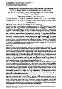
The high-level model is shown in Figure 9. Simulink represents models as block diagrams where directed arrows represent the ow of time-varying scalar (thin lines) or vector (thick lines) signals. Each block represents a function which operates on the signal. The leftmost block performs the integration of the object's motion. The constants of motion are its input, and its outputs are the position and angle of the object. It contains state information about the current position, orientation, and speed of translation and rotation of the object. The mux block combines the position vector and angle scalar signals into a single 3-element vector. The \Compute Supports" block contains an external function which uses the object's position and orientation and returns a \mask" vector, which is a list of ones and zeroes representing the support state of each cell. This mask feeds into the rightmost block which checks if the mask has changed, and if so, recalculates the constants of motion. The updated constants feed back into the motion integration block as the set of supports changes. The details of the \Integration Of Object Dynamics" block are shown in Figure 10. The constants of motion, which are fed back as a single vector, are split up into components corresponding to each constant (either vector or scalar). The appropriate constants are used in conjunction with the object's current position and velocity to calculate the total force (f~) and total torque ( ). The \f" and \tau" blocks involve the multiplication and addition of the constants and position and velocity signals according to Equations 18 and 23. The details of these blocks are not presented here. The force and torque signals are then used in an expression of Newton's law to produce the linear and rotational accelerations by dividing by the mass and inertia of the object. The accelerations are then integrated twice to produce the velocities and position and orientation of the object. The details of the \Check for Change of Supports and Recalculation" block are shown in Figure 11. The mask vector feeds through a memory block to produce the mask vector at the \previous" time step.1 The block compares the previous value of the mask to the current value, and if they are dierent, the Recalculate block is triggered. When triggered, this block generates new values of the constants of motion according to their de nitions in Equations 18 and 23. 1 The memory block does not maintain a constant step size. It is updated along with the simulation as the step size changes dynamically to nd the exact time of transition. Thus there is not a true previous time.

14

Figure 10: Details of the \Integration of Object Dynamics" block. This block uses the constants of motion to compute the forces on the object and then applies Newton's law to integrate the motion.

Figure 11: Details of the \Check for Change of Supports and Recalculation" block. The memory and not equal blocks check for a change in supports. A change triggers the recalculate block to update the constants of motion.

15

0.2 0.1 0 -0.1

orientation (rad)

position (m)

PSfrag replacements x y

0

2

4

0

2

4

6

8

10

6

8

10

1.5 1 0.5 0

time (s)

Figure 12: Simulation of an elliptic-like eld. An overhead view (left) and a time plot of X~ cm and  (right). In the left plot, the object starts in the upper right and is transported to the center.  in this plot represent the positions of the cells, and arrows eminating from the  represent the vector whose components are the wheel speeds of each cell. The curved line traces the path of the center of the object. To run the model, a startup script de nes the positions and velocities of the cells, the size, weight, and initial conditions of the object, the coecient of friction, the length of simulation, etc. Simulink saves signals from the simulation for plotting and animation after the simulation runs.

4.2 Simulation Results

The simulator is capable of running test cases on any eld with constant wheel velocities, since both the cell positions and wheel speeds are inputs to the model. In this paper, we present results from two classes of elds on regular square-lattice arrays. The rst is an elliptic eld, de ned by the following equation.

V=

k

sxx

0

0

ksyy



X

(29)

This eld has the special property that the translational constants of motion, ks and f~o are invariant with respect to the set of supports[9]. In particular ks is diagonal (with elements ksxx and ksyy ) and f~o is everywhere zero. Therefore, the object acts as a simple mass-spring-damper system centered at the origin over the entire array. This eld also tends to orient a rectangular object such that its major axis aligns with the x axis of the array. In the limit of an in nitely dense array, the object exactly aligns itself with the array.[5] The results of a typical simulation of an elliptic eld are shown in Figure 12. Note the second-order underdamped dynamics in both the x and y directions. The object comes to rest in an orientation that is very close to aligned with the array (but not quite). Figure 13 shows the results of a very similar simulation to that in Figure 12. In both these simulations, the eld is the same, but the dimensions of the object are slightly dierent. In the second simulation, the translations of the object are the same, but the object comes to rest at an orientation well o of zero. This misalignment is a result of the discrete nature of the array[14], and is not an artifact of the simulation. This behavior is not predicted by continuous eld theory. A dierent type of eld, called a \squeeze" eld is used in the simulation shown if Figure 14. This eld is de ned such that all cells with positive y coordinate push on the object in the negative y direction, and all cells 16

0.2 0.1 0 -0.1

orientation (rad)

position (m)

PSfrag replacements x y

0

2

4

0

2

4

6

8

10

6

8

10

1.5 1 0.5 0

time (s)

Figure 13: Simulation of the same eld with an object of slightly dierent size. An overhead view (left) and a time plot of X~ cm and  (right). with negative y coordinate push in the positive y direction. Such a eld tends to \squeeze" an object in a manner similar to that of a parallel-jaw gripper. Under such a eld, a rectangular object will move to the x axis and align its major axis with the x axis.[2] In this simulation, the object moves to the x axis, but comes to rest in a non-zero orientation. Again, this misalignment is due to the discrete nature of the array and is not predicted by continuous eld theory. Note that the translational dynamics for the squeeze eld are piecewise second order rather than purely second order for the elliptic eld.

5 Discussion In this paper, we introduced the Modular Distributed Manipulator System, a variation of several microscale MEMS manipulators with signi cantly greater control, computation, and communication capabilities. The paper developed the dynamic models of objects transported on discrete actuator arrays under several dierent contact models. Unlike previous approaches, the models speci cally accounted for the nite number of contact points. Depending on the contact model, the resulting dynamics were piecewise linear rst order or second order. r to investigate the motion Based on these models we developed a powerful simulator program using Simulink of objects of various sizes on various velocity elds. The simulations demonstrate dynamic responses not predicted by prior work of other researchers which used continuous eld approximations to discrete actuator arrays. In particular, the simulations showed that objects with slightly dierent dimensions can have very dierent stable orientations. This topic will be the subject of a future paper. This result indicates that open-loop operation of actuator arrays are not sucient to accurately control the motion of objects, and that closed-loop control may be necessary. While this paper focused only on open-loop operation the modeling in this paper can be applied to closed-loop operation where the wheel velocities are updated as the object moves. With changing wheel speeds, the dynamics will no longer be piecewise constant, but the instantaneous forces acting on an object are properly represented by the equations in this analysis. The results in this paper can be used to predict the stability and convergence of closed-loop control schemes. This is the topic of future work. 17

-0.5

0.2 0.1 0 -0.1

orientation (rad)

position (m)

PSfrag replacements x y

0

2

4

0

2

4

6

8

10

6

8

10

1.5 1 0.5 0

time (s)

Figure 14: Simulation of a squeeze-like eld. An overhead view (left) and a time plot of X~ cm and  (right).

References [1] S. Akella, W. Huang, K.M. Lynch, and M.T. Mason. Sensorless parts feeding with a one joint robot. In Proceedings. Workshop on the Algorithmic Fundamentals of Robotics, 1996. [2] K.F. Bohringer, B.R. Donald, R. Mihailovich, and N.C. MacDonald. A theory of manipulation and control for microfabricated actuator arrays. In Proceedings. IEEE International Conference on Robotics and Automation, 1994. [3] M. Erdmann. An exploration of nonprehensile two-palm manipulation: Planning and execution. In Proceedings. Seventh International Symposium on Robotics Research, 1995. [4] K.Y. Goldberg. Orienting polygonal parts without sensors. Algorithmica: Special Issue on Computational Robotics, 10:201{225, August 1993. [5] L. Kavraki. Part orientation with programmable vector elds: Two stable equilibria for most parts. In Proceedings. IEEE International Conference on Robotics and Automation, 1997. [6] J. Luntz, W. Messner, and H. Choset. Parcel manipulation and dynamics with a distributed actuator array: The virtual vehicle. In Proceedings. IEEE International Conference on Robotics and Automation, 1997. [7] J. Luntz, W. Messner, and H. Choset. Virtual vehicle: parcel manipulation and dynamics with a distributed actuator array. In Proceedings of SPIE vol. 3201. Sensors and Controls for Advanced Manufacturing. International Symposium on Intelligent Systems and Advanced Maufacturing., 1997. [8] J. Luntz, W. Messner, and H. Choset. Stick-slip operation of the modular distributed manipulator system. In Proceedings. AACC American Controls Conference, 1998. [9] J. Luntz, W. Messner, and H. Choset. Velocity eld design on the modular distributed manipulator system. In Proceedings. Workshop on the Algorithmic Foundations of Robotics., 1998. [10] J.E. Luntz and W. Messner. The virtual vehicle - a materials handling system using highly distributed coordination control. In Proceedings. IEEE Conference on Control Applications, 1995. 18

[11] J.E. Luntz and W. Messner. Work on a highly distributed coordination control system. In Proceedings. AACC American Controls Conference, 1995. [12] J.E. Luntz and W. Messner. The virtual vehicle: Materials handling using distributed actuation and highly distributed coordination control. In Proceedings. Japan-USA Symposium on Flexible Automation, 1996. [13] J.E. Luntz and W. Messner. A distributed control system for exible materials handling. IEEE Control Systems Magazine, 17(1), February 1997. [14] J.E. Luntz, W. Messner, and Choset H. Open loop orientability of objects on actuator arrays. In To Appear In Proceedings. IEEE International Conference on Robotics and Automation, 1999.

A Appendix: Derivations of Other Friction Modes

A.1 Coulomb Friction

The force from each cell under Coulomb friction is f~iC

 

= sign V~i

(30)

Ni :

The total force is the sum of f~iC over all the cells. The expression of the total force, using inner product summation, is ~: f~C = sign (V) N (31) Substituting the expression for N~ from Equation 13 into Equation 31 leads to f~C

20
? = W sign (V) BT BBT ?1 4 1

3 5 X~ cm {z } | k 213 ?
+ W sign (V) BT BBT ?1 4 0 5 0 {z } | 0 0 0 1

s

= ks C X~ cm + f~oC

C

f~oC

(32)

This represents the dynamics of a mass-spring system without damping. The spring constants and oset force are dierent than those obtained from a viscous friction model. The derivation of rotational dynamics under Coulomb friction is similar. The torque from each cell is iC

=

~

Xi

 



? X~ cm  sign

~ 

Vi Ni

 

 

= X~ i  sign V~i ? X~ cm  sign V~i

Ni :

(33)

De ne Ri C = X~ i  sign V~i , which de nes the components of the vector R~ C . The expression for the total torque using inner product summation is C

= R~ C N~ T ? X~ cm  sign (V) N~ T : 19

(34)

Substituting the expression for N~ from Equation 13 into Equation 34 leads to C

213 ?
? 1 = W R~ C BT BBT 405 |

0

{z

} 20 03
? ? 1 + W R~ C BT BBT 41 05 X~ cm 01 {z } | ~k   +X~ cm f~oC+ks C X~ cm ~C C ~  C ~C ~ o C

C s

= o + ks Xcm ? fo +ks

 X~ cm

Xcm

(35)

which is also similar to the viscous case but without damping.

A.2 No-Slip Friction

The force from each cell with no-slip contact is Km G fiNx = rix ?Vix Rm

| {z } foNix

 |

Bm +

Km 2 Rm

{z

+



Km G ; Rm

}

bN

(36)

Since the wheels are rolling with the object, we can substitute the actual speed of the object at cell i in the previous equation and vectorize the x and y components. f~iN

= f~oNi

?

_

~ cm + ! X



0 1 ?1 0



~i X

?

~ cm X



bN

(37)

This represents a constant force per cell with damping. This equation can then be summed over all the cells under the object to produce a net force on the object. For n cells supporting the object, the expression is f~N

=

 0 1  X  X ~N N ~_ N ~ i ? nX ~ cm X ? !b X fo ? nb cm ?1 0 | {z } |{z} B ~f  0 1  X  _ i

N o

N

= f~oN ? B N X~ cm ? !bN ?1 0

~i X

? nX~ cm

The rotational dynamics under no-slip friction are not presented here, but are derived similarly.

20

(38)