DESIGN OF A FRACTIONAL CONTROL USING PERFORMANCE CONTOURS. APPLICATION TO AN ELECTROMECHANICAL SYSTEM A. Oustaloup 1 , V. Pommier 2 , P. Lanusse
3
Abstract The article uses complex fractional differentiation to design a controller ensuring dynamic behavior of a control system. The proposed method uses two contours called “performance contours” and constructed on the Nichols diagram. The first contour is the common Nichols magnitude contour that can be considered as an iso-overshoot contour. The second contour constructed thanks to complex fractional differentiation is a new contour defined on the Nichols diagram and parameterized by the damping ratio. The design method leads to the computation of a complex fractional order transfer function whose open-loop Nichols locus tangents both performance contours, thus ensuring stability margins and dynamic behavior. The method is applied to a DC motor whose speed is controlled. Mathematics Subject Classification: 26A33 Key Words and Phrases: fractional differ-integration, optimization, control system, dynamic behavior
∗
Published in ”Fract. Calc. Appl. Anal.”, 6, No 1 (2003), 1-24; visit the websites: www.math.bas.bg/˜fcaa , www.diogenes.bg/fcaa
2
A. Oustaloup, V. Pommier, P. Lanusse 1. Introduction 1.1. Motivations of the article
The article proposes an application of the complex fractional integrator to control system design. Indeed, the compactness of fractional calculus is used here to compute a controller with a method based on an optimisation with few parameters. The aim of the control system is to ensure dynamic performance. Dynamic performance are well-known in the time-domain: the settling time ts , the overshoot in percent O%, the damping ratio ζ. For a simple second-order system, these characteristics are linked all together. The question is to know whether it is possible to compute a controller that achieves all three dynamic performance for any linear system whatever its order. As many design methods are based on a frequency-domain approach, a method that answers this question is researched in the frequency domain. As it is well-known that the overshoot in percent is strongly correlated to the resonant peak of he complementary sensitivity function (even if the system is not a second order system), the overshoot in percent is easily guaranted using frequency domain loop-shaping. As it is well-known that the settling time is strongly correlated to the closed-loop cut-off frequency and thus the open-loop gain crossover frequency, the settling time is also easily guaranted using frequency domain loop-shaping. Concerning the damping ratio, it is generally not linked to the resonant peak of he complementary sensitivity function for systems with an order other than 2. Nevertheless it would be convenient to have an equivalent of the damping ratio in the frequency-domain. In this article, it is shown how complex fractional differentiation have already been used to give an equivalent of the damping ratio in the frequency domain. Then we propose a new method, also in the frequency-domain, to compute a controller to ensure at the same time the overshoot, the damping ratio and the settling time of the response of a control system whatever the desired values of these parameters. This method is based on complex fractional differentiation. 1.2. Specific contributions of the article To develop the proposed method in the frequency domain, and more particularly with Nichols locus, it is first of all necessary to have an equivalent of the time-domain specifications in the frequency domain.
DESIGN OF A FRACTIONAL CONTROL USING . . .
3
It has been shown previously that, in the case of an unlimited rectilinear open-loop Nichols locus, the magnitude peak, M t , is indicative of the overshoot in percent O% [8],[12]. A Nichols diagram magnitude contour can thus be considered as an iso-overshoot contour (see Appendix entitled “Parametrization of a magnitude contour by the corresponding overshoot in percent”). Also, still in the case of an unlimited rectilinear open-loop Nichols locus, some new contours indicative of the closed-loop damping ratio ζ have been built using complex fractional differentiation [8],[9]. The construction method is summarized in Section 2. The interest of these contours is that their application domain oversteps this study context. We showed that these contours are valid, on the one hand in the case of limited rectilinear behavior around the gain cross-over frequency, and on the other hand, in the case of limited curvilinear behavior with an admissible degree of concavity. Both contours, the magnitude (or iso-overshoot) contour and the isodamping contour, define performance contours. To ensure dynamic performance, this paper introduces a method to design an open-loop transfer function whose Nichols locus tangents both performance contours. To simplify computation, complex fractional (or non integer) order transfer function is used since it can be defined with few parameters. For minimum-phase plants, the controller is then obtained from the ratio of this open-loop transfer function to the plant transfer function. This way to obtain the controller can be extended to unstable or non-minimum-phase plants, and also plants with bending modes, and discrete-time problems [7]. 1.3. Organization of the article In Section 2, a geometrical construction method for a chart of isodamping contours is given, using complex non-integer integration [5],[13]. It uses an envelope technique on the Nichols diagram for a set of segments of the open-loop Nichols locus, which are called generalized templates, and each providing the same closed-loop damping ratio. This section also introduces the transfer function of a complex non-integer integrator which defines the generalized template. Section 3 first shows how to use the charts of performance contours. An analytic expression of each contour is provided, and the equations of tangents to the contours are given. Then the open loop transfer is defined. The study of this transfer leads to the computation of its magnitude and phase and provides the equation of the tangent to its Nichols locus.
4
A. Oustaloup, V. Pommier, P. Lanusse
Section 4 describes a two-step method to compute an open-loop transfer function whose Nichols locus tangents both performance contours. A preliminary computation consists in computing the straight line which tangents both performance contours, and called common tangent. Then, the first step of the method is to render equal this common tangent to the tangent to the open-loop Nichols locus at gain crossover frequency ωcg . This step is conditioned by the hypothesis that the rectilinear part of this Nichols locus is long enough to tangent both a magnitude contour and an isodamping contour. To check this hypothesis, some parameters which influence the length of the rectilinear part of the Nichols locus must be chosen. To avoid choosing them, the second step of the method proposes a different approach to the problem. It leads to solve a nonlinear system by minimizing a cost function under equality and inequality constraints and using the results of the first step as initial conditions. Finally, in Section 5, the proposed approach is applied to an electromechanical system. The different steps of the computation to obtain an openloop transfer function whose Nichols locus tangents two required performance contours are detailed. Then the controller is computed and implemented. Experimental results are given. 2. Complex non-integer integration and isodamping contours 2.1. Generalized template and non-integer integration The generalized template is an any-direction segment around the gain cross-over frequency ωcg on the Nichols diagram. It is an extension of the vertical template that represents a vertical segment around ωcg . This vertical template is achieved using a real non-integer (or fractional) integration order, n, which defines its phase placement at -n90◦ for the gain crossover frequency ωcg (Figure 2). It is described by the open-loop transfer function of a real non integer integrator: β (s) =
³ ω ´n cg
s
for ω ∈ [ωA , ωB ], n ∈ R.
(1)
By extension, the generalized template can then be characterized by a complex non-integer integration order, n. The real part defines its phase placement at −Re(n)90◦ for ωcg , and the imaginary part defines its angle to the vertical (Figure 2). The generalized template is then a priori defined
DESIGN OF A FRACTIONAL CONTROL USING . . .
5
by the real part (with respect to imaginary unit i) of the open-loop transfer function of a complex non integer integrator: h³ ω ´n i cg for ω ∈ [ωA , ωB ] , n ∈ Ci . (2) β (s) = Re/i s The imaginary unit i of the integration order n (n = a + ib) is independent of the imaginary unit j of the variable s (s=σ+jω). A posteriori, to ensure |β(jωcg )| = 1 and so that the sign of the imaginary integration order b has an effect on the sign of the phase slope of the¡ Nichols ¢ d π locus of β(s) at ωcg ( dlogω arg β ◦ (jω) ω=ωcg = − 180 π ln (10) b tanh b 2 ), it is necessary to describe the generalized template by the transfer function: ·³ ¸¶−sign(b) ³ ³ π ´´sign(b) ³ ω ´a µ ωcg ´ib cg β (s) = cosh b Re/i . 2 s s
(3)
Note: The phase placement of the Nichols locus of β(s) at ωcg (arg β ◦ d (jωcg ) = −a90◦ ) and the gain slope at ωcg ( dlogω |β (jω)| ω=ωcg = −20a) depend exclusively on the real integration order a. 2.2. Generalized template envelope as isodamping contour The easiest geometrical way to construct an isodamping contour is to use an envelope technique. The contour is then defined as the envelope tangented by a set of segments (Figure 3). On the Nichols diagram, each segment of the set can be considered as the rectilinear part of an open-loop Nichols locus that ensures the closed-loop damping ratio value corresponding to the contour. The rectilinear part of the open-loop, around gain crossover frequency ωcg is the “generalized template” of third generation CRONE control (Section 2.1 and [10]). The closed-loop damping ratio characterizes the decrease rate of the overshoot of the step response. It is given by the cosine of half the angle formed at the origin of the complex plane by the complex-pole pair from which this mode results. When a response has several oscillatory modes, there are as many damping ratios as there are modes. The damping ratio of the dominant mode is the one used to quantify the stability degree of the closed-loop. In this context, the complex-poles pairs from which the closed loop oscillatory mode results, is the solution of the closed-loop characteristic equation (1 + β(s) = 0) whose open-loop Nichols locus traces a generalized template (i.e. an any-direction segment around frequency ωcg ).
6
A. Oustaloup, V. Pommier, P. Lanusse
Closed-loop dynamic behavior is essentially linked to the open-loop behavior around ω cg . So, determining a transfer function which describes the generalized template is enough to establish the characteristic equation indicating the dynamics, and thus the damping. 2.3. Analytic study of performance contours and of the fractional open-loop transfer function 2.4. Magnitude contours The analytic expression of a magnitude contour is determined from a point M on the Nichols diagram P . If X and Y, expressed in degrees and in decibels, are the cartesian coordinates of M , its polar coordinates (modulus and argument) are respectively defined by: Y
ρ = 10 20
and θ =
π X. 180
The affix of M , β(jω), can then be written: ³ π ´i h ³ π ´ Y X + jsin X . β (jω) = 10 20 cos 180 180
(4)
(5)
For a Nichols magnitude contour parameterized by M t and called ΓM t , β(jω) is such that: ¯ ¯ ¯ β (jω) ¯ ¯ ¯ (6) ¯ 1 + β (jω) ¯ = Mt . Using a more condensed form, ΓM t is defined by : ( ) Y 10 10 2 . ΓM t = M (X, Y ) ∈ P, ¡ π ¢ Y Y = Mt 20 10 1 + 2.10 cos 180 X + 10
(7)
The equation of the tangent to ΓM t at point (X i , Y i ) is deduced from relation (7) and can be written: Y = α1 X + β1 .
(8)
DESIGN OF A FRACTIONAL CONTROL USING . . .
7
2.5. Isodamping contours Isodamping contours result from a construction using the envelope technique (Section 2.2) and are thus only defined graphically. To define the contours analytically, a polynomial equation is determined by interpolation of graphical data of each contour. The isodamping contour parameterized by ζ, and called Γζ is then defined by the following equation: Γζ : X =
2 X
fj (ζ) Y 2j withfj (ζ) =
j=0
3 X
ajk ζ k ,
(9)
k=0
X and Y being the coordinates, always expressed in degrees and in decibels, and ajk the coefficients given in Table 1: j/k 0 1 2
0 -180.36 -1.1538 -0.0057101
1 117.7 3.888 0.0800962
2 -74.316 -5.2999 -0.0060354
3 40.376 2.5417 0.0016158
To use the same syntax as for a magnitude contour (relation 7), the contour Γζ is defined by: 2 X Γζ = M (X, Y ) ∈ P, X − fj (ζ)Y 2j = 0 , (10) j=0
The equation of the tangent to Γζ at point (X i , Y i ) is deduced from relation (10) and can be written: Y = α2 X + β2 .
(11)
2.6. Open-loop transfer including generalized template The aim of this section is to describe analytically, for a nominal plant, the open-loop behavior which takes into account: - the accuracy specifications at low frequencies; - the generalized template around frequency ωcg ; - the plant behavior at high frequencies in accordance with input sensitivity specifications for these frequencies.
8
A. Oustaloup, V. Pommier, P. Lanusse
For stable minimum-phase plants, this behavior can be described by the following transfer function (Figure 4): β(s) = βl (s)βm (s)βh (s).
(12)
• βm (s), based on complex non-integer integration, is the fractional transfer function describing the band-limited generalized template (Section 3.3.1 & [11]). • βl (s) is the rational transfer function of a order nl proportionalintegrator, whose corner frequency equals the low corner frequency of βm (s), so that joining βl (s) and βm (s) does not introduce extra parameters. βl (s) is defined by: ³ ωl ´nl . (13) βl (s) = 1 + s For accuracy specifications, nl has to be greater than or equal to the relative order npl of the plant at low frequencies (ωωh ), order nh is given by nh ≥ nph , with nh = nph ensuring invariability of the input sensitivity function with the frequency, and nh >nph ensuring decrease. 2.6.1. Transfer function describing the band-limited generalized template For a band-limited generalized template, relation (3) must be replaced by the more general expression: Ã !a !ib0 −q0 sign(b0 ) Ã s s 1 + ωh 1 + ωh Re/i C , (15) βm (s) = K 0 1 + ωs 1 + ωs l
l
so that the phase placement of the generalized template at frequency ωcg only depends on parameter a, the computation of the phase shows that Co must be equal to: "Ã ¶ ! Ã µ ¶ !# 12 µ ωcg 2 ωcg 2 / 1+ . (16) C0 = 1+ ωl ωh
DESIGN OF A FRACTIONAL CONTROL USING . . .
9
q’ is the smallest integer such that b0 verifies |b0 | < min (|b1 |, |b2 |) with : ¯ "µ ¶ #¯ ¯ π ωl 2 ¯¯ ¯ ¯ and |b2 | = π/ ¯ln C0 |b1 | = ¯¯ (17) ¯. ¯ ¯ ωh ln(C02 )¯ K is computed to get a 0 dB gain at frequency ωcg .
3. Tangency of the open-loop Nichols locus to two performance contours 3.0. Preliminary computation: equation of the common tangent to two performance contours The determination of the common tangent which tangents both a given magnitude contour and a given isodamping contour, requires the analytic expressions of each contour and of the equations of their tangent (relations 7,10, 8, 11). This common tangent can be defined by two points, M 1 (X 1 ,Y 1 ) and M 2 (X 2 ,Y 2 ), and thus from four coordinates which are the solutions of the system of equations: Y1 10 10 2 Y1 Y1 = Mt π 20 10 X1 )+10 1+2.10 cos( 180 2 P X2 = fj (ζ)Y22j . (18) j=0 α1 = α2 β =β 1
2
The first two equations express that the points M 1 and M 2 belong respectively to the contours ΓM t and Γζ (Figure 5), while the last two equations express the equality of the tangents to these contours (8,11). From the four solutions of (18), that is to say X 1 , Y 1 , X 2 and Y 2 , the equation of the common tangent can be written: Y = αT (X − XT ) .
(19)
10
A. Oustaloup, V. Pommier, P. Lanusse
3.1. First step The principle of the first step is conditioned by the hypothesis that the corner frequencies, ωl and ωh , must be far enough from each other so that the rectilinear part of the open-loop Nichols locus (which defines the generalized template) is long enough to tangent both a magnitude contour and an isodamping contour. In this study context, it is possible to interpret the generalized template as a part of the common tangent to both contours. The first step consists in determining the parameters of the open-loop transfer whose rectilinear part of the Nichols locus belongs to this common tangent, or, in other words, whose tangent to the Nichols locus at frequency ωcg is the same as the common tangent (Figure 6). As the common tangent equation is characterized by two parameters, only two parameters of the open-loop transfer function can be determined using the equality of this common tangent with the tangent to the open-loop Nichols locus. The others parameters need to be fixed. We choose to fix: - the gain crossover frequency, ωcg - the orders of the transfer functions βl (p) and βh (p), nl and nh - the corner frequencies, ωl and ωh . a and b0 are then computed by rendering equal the equation of the common tangent to the open-loop Nichols locus at frequency ωcg : a=
h π ³π ´ i 1 XT + nl − θcgl + nh θcgh , θcgh − θcgl 180 2
(20)
while b’ is the solution of equation: ¯ d|β (jω)|dB ¯¯ αT = . d arg β ◦ (jω) ¯ω=ωcg
(21)
Finally, K, computed to ensure a gain of 0 dB at frequency ωcg, is defined by: µ ¶ ¡ ¢ ωcg 2 20 log K = 10q 0 sign(b0 ) log(cosh2 b0 (θcgl − θcgb )) + 10a log 1 + ( ) ωl µ ¶ µ ¶ ωcg 2 ωl 2 − 10nb log 1 + ( ) − 10(a − nh ) log 1 + ( ) . (22) ωcg ωh
DESIGN OF A FRACTIONAL CONTROL USING . . .
11
3.2. Second step Although the first step has the advantage of being programmed easily while giving satisfactory results, it has the disadvantage of requiring an arbitrary choice of the corner frequencies ωl and ωh which may be incompatible with the performance requirements related to input sensitivity and disturbance rejection. Moreover, even if the open-loop Nichols locus tangency with performance contours is well-ensured around ωcg , outside this zone the Nichols locus may curve back across the contours. Therefore, the second step aims to compensate these disadvantages. It uses results from the first step, notably the coordinates of tangency points M 1 and M 2 . ♦ To avoid an arbitrary choice of ωl and ωh , the problem is set differently by considering the frequencies ω1 and ω2 that are defined as the frequencies such that the open-loop Nichols locus tangents the contours (Figure 6). Instead of trying to render equal the tangent to open-loop Nichols locus at ωcg and the common tangent to performance contours (first step), we can try to render equal tangents to open-loop Nichols locus at ω1 and ω2 and tangents to performance contours at M 1 and M 2 . As M 1 and M 2 are both on performance contours and on the open-loop Nichols locus, the coordinates of these points on the contours are equal to gains and phases of the open-loop frequency response at ω1 and ω2 . Thus: Y1 = |β(jω1 )| Y2 = |β(jω2 )| . (23) X1 = arg β(jω1 ) X2 = arg β(jω2 ) Also, as the open-loop Nichols locus tangents the performance contours at these points, the slopes α of the tangents to the magnitude and isodamping contours are equal to the slopes ∆(ω1 ) and ∆(ω2 ) of the tangents to the open-loop Nichols locus at frequencies ω1 and ω2 , thus: ½ α = ∆ (ω1 ) . (24) α = ∆ (ω2 ) Relations (23) and (24) constitute a set of six nonlinear equations. As gain crossover frequency ωcg and orders nl and nh of transfer functions βl (p) and βh (p) are fixed, the four parameters a, b0 , ωl and ωh must be determined to characterize completely the open-loop transfer. As frequencies ω1 and ω2
12
A. Oustaloup, V. Pommier, P. Lanusse
must also be computed, a system of six nonlinear equations in six unknowns is to be solved. It is solved using an optimization technique. As the aim is to ensure open-loop Nichols locus tangency to both contours and above all to guarantee equality, or at least near equality, of slopes, we chose to minimize: J = (∆(ω1 ) − α)2 + (∆ (ω2 ) − α)2 , (25) under four equality constraints: |β(ω1 )| = Y1 ,
|β(ω2 )| = Y2 ,
arg β(ω1 ) = Xd1 and arg β(ω2 ) = X2 . (26) ♦ To guarantee that the open-loop Nichols locus does not curve back across the magnitude contour and the isodamping contour (that it must only tangent), inequality constraints are added to the algorithm which computes the open-loop transfer function parameters. Concerning the magnitude contour: for each point (X, Y ) of the openloop Nichols locus, the closed-loop gain computed from relation (6) must be inferior or equal to required peak magnitude. Concerning the isodamping contour (Figure 7): for each point (X, Y ) of the open-loop Nichols locus, abscissa X of the Nichols locus corresponding to ordinate Y must be superior or equal to abscissa XΓς (relation 9) of the point of the isodamping contour corresponding to the same ordinate Y . 3.3. Frequency responses requirements So that the open-loop frequency configuration respects study conditions used to validate Nichols magnitude contours as iso-overshoot contours and to construct isodamping contours [8], this configuration must favor an closed-loop oscillatory mode. Thus, frequency responses in tracking mode and in disturbance rejection mode must show clear resonance. For given peak magnitudes M t and M r in tracking mode and in disturbance rejection mode, these responses must show the best selectivity around resonant frequencies ωrt and ωrr (Figure 8). Except within the zones of tangency to the magnitude contour and to the isodamping contour, the open-loop Nichols locus must curve away as much as possible from these contours. Also, the average slope of Nichols locus at frequency ωcg must not be slight. Indeed, if this slope is represented by a generalized template characterized by real order a and imaginary order b, the slope of the gain diagram
DESIGN OF A FRACTIONAL CONTROL USING . . .
13
around ωcg equals −6a dB per octave (Figure 9). Thus, considering template tangency to a performance contour (a Nichols magnitude contour or an isodamping contour), a slight slope of the template leads to a low value of a (Figure 10), and so to a gain slope (Figure 9) too slight to ensure: - a value of |β (jω) / (1 + β (jω))|dB near enough to 0 at frequencies inferior and close to ωcg (Figure 8a). |β (jω)| must thus be high compared to 1 (Figure 9). - a value of |1/ (1 + β (jω))|dB near enough to 0 at frequencies superior and close to ωcg (Figure 8b). |β (jω)| must thus be low compared to 1 (Figure 9). 4. Application to an electromechanical system 4.1. Experimental plant A test bench developed by the CRONE team of the LAP in 1995 is used. It is constituted of two identical parts with a rigid link between them. Each part is a DC motor driving a inertia disk. The output to be controlled is the shaft velocity provided from a quadrature encoder giving 10000 count per turn. When a single motor generates a torque, the transfer function of the plant which gives the velocity is: G(s) =
9092 . (1 + 0.0047s)(1 + 96s)
(27)
The two time constants of the model are far from each other since one is electrical and the other mechanical. 4.2. Performance specifications In the time domain, the dynamic specifications are: - O% overshoot in percent around 20 to 25% - ζ damping factor around 0.7, with a tolerance of ±5% - ωcg gain crossover frequency equal to 10 rad/s. The control law being designed in the frequency domain, such specifications must be translated into two performance contours. For the overshoot O%, the value of the peak magnitude M t must be determined so that a Nichols contour parameterized M t may be the iso-overshoot contour parameterized O%. A 20 to 25% overshoot corresponds to a value of M t of 2dB (see Appendix). For the damping factor ζ, we only have to consider the isodamping contour of parameter ζ.
14
A. Oustaloup, V. Pommier, P. Lanusse
4.3. Tangency of the open-loop Nichols locus to two performance contours ♦ Preliminary computation The coordinates of the tangency points resulting from the solving of the system of equations (18) are: - (-130.46◦ ; 7.48dB) for M 1 on the Nichols magnitude contour - (-123.85◦ ; 4.1dB) for M 2 on the isodamping contour. These values lead to the numerical tangent equation: YdB = −0.444(X ◦ − 113.62). ♦ First step Gain crossover frequency (ωcg = 10 rad/s), orders (nl = 2 and nh =3) of βl (s) and βh (s), and corner frequencies (ωl = 1 rad/s and ωh =100 rad/s) are fixed. It is then possible to determine the other parameters of β(s):
a = 1.11 ; b0 = 0.635 ; q 0 = 1 and K = 18.21. ♦ Second step This step uses the coordinates of the two tangency points of M 1 and M 2 of the first step to establish the nonlinear system of six equations (relations 23 and 24). It also uses the values of the open-loop transfer function parameters to initialize the algorithm to solve this problem. Gain crossover frequency ωcg , orders nl and nh of the transfer functions βl (s) and βh (s), and corner frequencies ωl and ωh, do not change with respect to the first step. The algorithm thus gives several open-loop transfer functions respecting the specifications. The one giving the highest corner frequency ωl favors disturbance rejection of the perturbation, and the one giving the lowest corner frequency ωh minimizes the effect of measure noise. For reasonable compromise, the selected solution is the one with the lowest ratio ωh/ ωl. The open-loop transfer function is then characterized by: a = 0.9675; b0 = 0.305; q0 = 4; K = 13.76; ωl = 0.98rad/s and ωh = 46rad/s. Figure 12 shows the obtained open-loop Nichols locus and we can verify its tangency to performance contours parameterized by M t and ζ.
DESIGN OF A FRACTIONAL CONTROL USING . . .
15
4.4. Controller The controller transfer function results from the ratio of the open-loop transfer function to the plant transfer function. Its expression is a complex non-integer transfer function. The design of the achievable rational controller consists in replacing this complex non-integer controller by an integer (or rational) order controller which has the same frequency response [10]. The discrete-time controller is obtained using Tustin transform with a sampling period of 5ms: 2.4892.10−8 z 2 + 4.9784.10−8 z + 2.4892.10−8 9.94125z + 9.94125 + + z 2 − 2z + 1 z−1 0.0557z 2 + 0.0083z − 0.0474 0.5435z + 0.5435 2.148z + 2.148 − − . z 2 − 1.6408z + 0.6759 z − 0.7183 z − 0.9969 (28)
C(z) =
4.5. Experimental results Figure 13 shows the step-response to a reference input signal of magnitude 20,000 (2 turn per second). Measured value of the overshoot is 25%. The specification concerning a required overshoot of 20 to 25% is thus respected. The damping factor is evaluated from the highest half-angle at the origin formed by the complex-poles pair of the fractional closed-loop transfer function. Computation of complex-pair poles [11] leads to ζ = 0.72, thus a relative error of 2.85% compared to designed damping factor, ζ = 0.7. 4.6. Conclusion The first part of this article (Section 2) presents the method for construction of isodamping contours by the envelope technique. This technique uses segments obtained using complex non-integer integration. Section 3 gives the formalism used in the design of the control law, in particular the equations of the tangents to the performance contours and to the open-loop Nichols locus. Section 4 defines the frequency-domain design method using tangency relations between the performance contours and the open-loop Nichols locus. The first step of this method is conditioned by a constraint on the openloop behavior at low and high frequencies. The second step of the method relaxes this constraint which can be prejudicial to performance at low and high frequencies.
16
A. Oustaloup, V. Pommier, P. Lanusse
Finally the example given in Section 5 shows the validity of the method. In a robust context, this method could be extended to frequency-domain robust design methods (QFT, CRONE,...) to limit either the upper value of the closed-loop overshoot or the lower value of the closed-loop damping ratio. In a QFT design [2],[3],[4], an overshoot contour or an isodamping contour can be graphically extended by taking into account the shape of the plant frequency uncertainty domains (called templates in a QFT design). In a CRONE design [7],[9], these contours can be used directly. References [1] J. J. D’A z z o and C. H. H o u p i s, Linear Control System Analysis and Design, Conventional and Modern. McGraw Hill, N. York (1988). [2] I. M. H o r o w i t z and M. S i d i, Synthesis of feedback systems with large plant ignorance for prescribed time-domain tolerances. International Journal of Control 16 (1972), 287-309. [3] I. M. H o r o w i t z, Survey of quantitative feedback theory (QFT). International Journal of Control 53 (1991), 255-291. [4] I. M. H o r o w i t z, Quantitative Feedback Design Theory - QFT. QFT Publications, Boulder - Colorado (1993). [5] K. S. M i l l e r and B. R o s s, An Introduction to the Fractional Calculus and Fractional Differential Equations. Wiley-Interscience Publ. (1993). [6] A. O u s t a l o u p, La d´erivation non enti`ere : Th´eorie, synth`ese et applications. Editions Herm`es, Paris (1995). [7] A. O u s t a l o u p, B. M a t h i e u, P. L a n u s s e, The CRONE control of resonant plants: application to a flexible transmission. European Journal of Control 1 (1995), 113-121. [8] A. O u s t a l o u p, B. M a t h i e u, P. L a n u s s e, Int´egration non enti`ere complexe et contours d’isoamortissement – Complex non integer integration and isodamping contours. APII 29, No 2 (1995). [9] A. O u s t a l o u p, B. M a t h i e u, La commande Crone du scalaire au multivariable. Editions Herm`es, Paris (1999). [10] A. O u s t a l o u p, J. S a b a t i e r, P. L a n u s s e, From fractal robustness to the CRONE Control. Fractional Calculus & Applied Analysis (An Internat. J. for Theory and Applications) 2 (1999). [11] A. O u s t a l o u p, F. L e v r o n, F. N a n o t, B. M a t h i e u, Frequency band complex non integer differentiator: Characterization and synthesis. IEEE Transactions on Circuit and Systems 7 (2000), 25-40.
DESIGN OF A FRACTIONAL CONTROL USING . . .
17
[12] V. P o m m i e r, A. O u s t a l o u p, P. L a n u s s e, Synthesis of a noninteger control loop using performance contours. In: IEEE /Med 2000, Greece, Patras, 17-19 July, 2000. [13] S. G. S a m k o, A. A. K i l b a s, O. I. M a r i c h e v, Fractional Integrals and Derivatives: Theory and Applications.Gordon and Breach Science Publishers (1993). Appendix Parametrization of a magnitude contour by the corresponding overshoot in percent The overshoot in percent O, between 0 and 1, which characterizes the Nichols magnitude contour may be given by the closed-loop first overshoot, where the closed-loop corresponds to the Nichols locus of a generalized template tangent to this contour. It is written: O = an2 + bn + c,
(29)
a = 79.195; b = −138.507 and c = 59.528,
(30)
with numerical values:
the integration order n (between 1 and 2) –nπ/2 being the abscissa of the tangency point. Given that an n order generalized integrator leads to a magnitude peak of the form [13]: 1 Mt = , (31) sin nπ 2 it is possible to express n according to M t : 2 1 n = arcsin , (32) π Qa with
π 1 π < arcsin = n < π since 1 < n < 2, 2 Qa 2 then, including this expression in that of the overshoot: µ ¶ µ ¶ 2 1 2 2 1 O=a arcsin +b arcsin + c. π Qa π Qa
(33)
(34)
This relation provides a formula of O which permits a Nichols magnitude contour to be parameterized directly by an overshoot value from parameter M t expressed in decibels.
18
A. Oustaloup, V. Pommier, P. Lanusse FIGURES
Figure 1: Elementary control loop structure
Figure 2: Representation of the vertical template by a vertical segment in the Nichols diagram and of the generalized template by a segment with any direction in the Nichols diagram
DESIGN OF A FRACTIONAL CONTROL USING . . .
19
Figure 3: Envelope defining an isodamping contour in the Nichols plane
Figure 4: Different parts of the open-loop Nichols locus
20
A. Oustaloup, V. Pommier, P. Lanusse
Common tangent : Y = α X + β with α = α1 = α2 and β = β 1 = β
Tangent to the magnitude contour: Y = α 1X + β 1
ΓM t
M1(ω1)
Γζ
Gain (dB) 2
X2
Y1
X1 M 2 (ω 2)
Phase (degrees)
Y2
Tangent to the isodamping contour: Y = α 2X + β 2
Figure 5: Common tangent to performance contours
DESIGN OF A FRACTIONAL CONTROL USING . . . Open-loop Nichols locus
Gain (dB)
Common tangent to ΓMt
performance contours
Generalized template Γζ
Phase (degrees)
ωu
Figure 6: Illustration of the first step
Figure 7: Coordinates concerning the isodamping contour
21
22
A. Oustaloup, V. Pommier, P. Lanusse Mt 0dB (a)
~0 high β for ω < ωcg
Mr
ωrt ωcg
1 / (1 + β (jω )) dB
0dB (b)
ω
~0
ωcg ωrr
low β for ω > ωcg
ω
Figure 8: Gain diagrams in tracking (a) and regulation (b)
Figure 9: Open-loop gain diagram around ωcg
DESIGN OF A FRACTIONAL CONTROL USING . . .
23
Figure 10: Templates tangent an isodamping contour: their slight slope leads to a low value of a
Figure 11: CRONE team test bench
24
A. Oustaloup, V. Pommier, P. Lanusse
Figure 12: Open-loop Nichols locus tangenting a magnitude contour and an isodamping contour
Figure 13: Experimental results 1
Laboratoire Automatique et Productique - Universit´e Bordeaux 351, Cours de la Lib´eration Received: June 25, 2002 33405 Talence, FRANCE e-mail:
[email protected] 2
ENSICA - 1, Place E. Blouin - 31 056 Toulouse, FRANCE e-mail:
[email protected] 3
Revised: February 5, 2003
Laboratoire Automatique et Productique - Universit´e Bordeaux 351, Cours de la Lib´eration 33405 Talence, FRANCE e-mail:
[email protected]