Design of an FPGA-Based FDTD Accelerator ... - Tohoku University

Int'l Conf. Par. and Dist. Proc. Tech. and Appl. | PDPTA'14 |

371

Design of an FPGA-Based FDTD Accelerator Using OpenCL Yasuhiro Takei, Hasitha Muthumala Waidyasooriya, Masanori Hariyama and Michitaka Kameyama Graduate School of Information Sciences, Tohoku University Aoba 6-6-05, Aramaki, Aoba, Sendai, Miyagi, 980-8579, Japan Email: {takei, hasitha, hariyama, kameyama}@ecei.tohoku.ac.jp

Abstract— High-performance computing systems with dedicated hardware on FPGAs can achieve power efficient computations compared with CPUs and GPUs. However, the hardware design on FPGAs needs more time than the software design on CPUs and GPUs. We designed an FDTD hardware accelerator using the OpenCL compiler for FPGAs in this paper. Since it is possible to design a hardware automatically from an OpenCL code, we can implement applications on FPGAs in a short time compared with the design by using a hardware description language. According to the result of the implementation of the FDTD accelerator on the FPGA, the processing speed is faster than a CPU. Moreover, its power consumption is about onetenth of a GPU. Keywords: OpenCL, FPGA, FDTD method, Hardware accelerator

1. Introduction In the field of the high performance computing such as three-dimensional image processing, electromagnetic simulation, fluid dynamics and DNA sequence, a very large scale computing system is required. However, the power consumption of high performance computer systems becomes a serious problem. The FPGA is attracting attention as the accelerator for such highperformance computing systems. A very large scale architecture for high performance computings can be implemented on a FPGA because of the advancement of the process technology. The power consumption of FPGAs is about one tenth as much as that of GPUs. However, very long time is required for the implementation of the FPGA-based accelerator. The software-based design on CPUs and GPUs needs only a software code by using C language or CUDA. On the other hand, the hardware-based design on FPGAs needs circuit modules for calculations, controls and

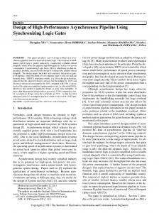
connecting to the host PC by using a hardware design language(HDL). To solve this problem, Altera Corporation released Altera SDK for OpenCL [1] which is the OpenCL compiler for FPGAs. OpenCL is the programming language for parallelized heterogeneous multicore architectures. OpenCL is standardized by the Khronos group [2]. The source code of the OpenCL is constituted by the host code and kernels. The initialization, the data-transfer from the host PC to the accelerator and running the kernels are described in the host code. The parallelized computation on the accelerator is described in the kernel code. As a feature of the OpenCL, the common source code can be run on the different architectures by using compilers corresponding to architectures such as multi-core CPUs, GPUs, the CELL processors and so on. In order to implement the OpenCL code on the FPGA board, Altera SDK for OpenCL can be used. This compiler does not require the HDL design for the calculation and connecting to the host PC by PCI express as shown in Fig.1, and the design time can be reduced. In the recent studies of the FPGA-based accelerator by using OpenCL, fractal image processing [6] and AES encryption encoding [7] have been reported. These studies achieve a low power and high performance computing compared with GPUs. In this article, we implement the FDTD (FiniteDifference Time-Domain) method accelerator by using the OpenCL compiler for FPGAs. We compare the performance of the FPGA-based accelerator with a CPU and a GPU in order to research the utility of the OpenCL compiler.

2. Implementation of an FPGA-Based FDTD accelerator by using OpenCL The FDTD method[3] has been widely used in an electromagnetic simulation. Since the FDTD method

372

Int'l Conf. Par. and Dist. Proc. Tech. and Appl. | PDPTA'14 |


  




  
  

  


 

 

  
               



  



 

Ezn+1 (i, j) = Ezn (i, j) n n+ 1 o n+ 1 −Py (i, j) Hx 2 (i, j + 1/2) − Hx 2 (i, j − 1/2) n n+ 1 o n+ 1 +Px (i, j) Hy 2 (i + 1/2, j) − Hy 2 (i − 1/2, j) (1)



!"

Fig. 1: OpenCL implementation on the FPGA has the high degree of parallelism, there are many studies which use computer clusters, GPUs [4], [5] and FPGAs [8]，[9] to accelerate the FDTD method. Figure 2 shows the flowchart of the FDTD method. It starts with transferring initial data of the electric and magnetic fields. Then the initial data are processed to obtain the electric field information for the first time step. After that, the boundary conditions are applied. Then the magnetic field information are obtained and the boundary conditions for the magnetic field are applied. These steps are repeated for a given number of time steps. Equation (1) shows the electric field computation. Equations (2) and (3) show the magnetic field computation. Electric and magnetic fields in x, y, z directions are denoted by E and H respectively. The time step is denoted by n and the coordinates of the 2D fields are denoted by i and j . Note that the boundaries of the electric and magnetic fields are calculated differently. Parameters P x, P y, Qx, Qy are determined by the permittivity, the permeability, the size of grids and the length of the time step. A detailed description of the FDTD is given in [3].



Fig. 2: The flowchart of the FDTD method

n+ 21

Hx

n− 21

(i, j + 1/2) = Hx

(i, j + 1/2)

−Qy (i, j) {Ezn (i, j n+ 21

Hy

n− 21

(i + 1/2, j) = Hy

+ 1) − Ezn (i, j)}

(i + 1/2, j)

−Qx (i, j) {Ezn (i

+ 1, j) − Ezn (i, j)}

(2)

(3)

Figure 3 shows the example of the OpenCL code for computing the electric field by Eq.(1). Thanks to the descriptions of global_id(0) and global_id(1) in line 4 and 5 respectively, the electric and magnetic fields in the coordinates of the two-dimensional fields are accessed in parallel. In this implementation, we make four kernel codes for updating electric fields, updating magnetic fields, applying boundary conditions and exciting electric fields. Counting time steps and running kernels are controlled by the host code. Let us explain about data-transfers between a host PC to accelerators. At the first of the FDTD computation, initial values of electric fields and magnetic fields, and the values of P x, P y, Qx, Qy are transferred from a host PC to accelerators. The values of excited electric fields are also transferred in every time step. When the value of time steps reaches the given value, the results

Int'l Conf. Par. and Dist. Proc. Tech. and Appl. | PDPTA'14 |

373

&

  

   

   

   

   

    1 

 
 
  !"#$! 2

 %
 
 & !"#$! 3 4 / 0

5 & .



'&(( %'& )%*+ ,)%*+ ,-)%*+ , )%*+ ,-) %-&*+ ,+)%*+ , )%*+ ,-)%*+ -&, .

Fig. 3: An example of the OpenCL code

of the simulation are transferred from accelerators to a host PC.

3. Evaluation We implement the FDTD method by C language on "Intel Core i7 920", and by OpenCL on "nVidia Geforce GTX 580" and "Nallatech P385-A7 FPGA board"[10]. This FPGA board has the Altera StratixV GX A7，a DDR3-SDRAM(8GB) and a PCI-Express. We use Visual Studio 2010(64bit) and nvidia GPU computing SDK 4.2 for the compilation on the CPU and the GPU. We use Altera SDK for OpenCL 13.0 for the compilation on the FPGA. Figure 4(a) shows the simulation model. This model has N × N grids (N=128,256,512). The electric field at (N/2,N/2) is excited as shown in Fig.4(b). The boundary area is a perfect conductor (Ez = 0). The single-precision floating-point is used for the simulation. Table 1 shows the resource usage on the FPGA. The number of processing units and the degree of the kernel vectorization can be changed [11]. When the kernel vectorization is used, each scalar operation in the kernel, such as addition or multiplication, is translated to an SIMD operation by the compiler. The processing units becomes smaller, and the throughput becomes higher. Figures 5(a),5(b) and 5(c) show the results of the simulation of the electric field on the CPU, the GPU and the FPGA, respectively. As shown in these figures, the simulation results are almost consistent with each other. However, there are very small errors since the rounding of a floating point are different depending on the platforms. Table 2 shows the processing time of the FDTD

method. The processing time of the FPGA is about half of that of the CPU. However, the processing time of the FPGA is about 22 times longer than that of the GPU. One of the main reasons is the bandwidth of the global memory. The bandwidth on the FPGA board is further narrower than that of the GPU board. In order to increase the performance on the FPGA, the memory access to the global memory should be reduced by improving the OpenCL code. The power consumption of the FPGA is 25W [6]. This power consumption is about one tenth of that of GPU board. Based on these results, the FPGA accelerator can achieve very low power and high performance computing if the OpenCL code is improved to reduce the memory access.

4. Conclusion In this article, we implement the FPGA-based accelerator for the electromagnetic simulation by using the OpenCL compiler. The processing time of FPGA is about half of that of CPU. However, the processing time is longer than that of GPU. The power consumption of the FPGA is about one tenth of that of GPU. For the future work, we improve the specialized OpenCL code for the FPGA. For example, the resource usage of processing units becomes small if the fixed-point calculation is used. Moreover, we are now designing the FPGA-based accelerator for the electromagnetic simulation on antennas and optical devices.

Acknowledgement This work is supported by JSPS KAKENHI grant number 24300013.

374

Int'l Conf. Par. and Dist. Proc. Tech. and Appl. | PDPTA'14 |

PEs 1 4 16(Vectorization)

Grids 128×128 256×256 512×512

Table 1: Resource usage LEs FFs 76965(16%) 127326(14%) 144072(31%) 302233(32%) 204092(44%) 435734(46%)

RAMs 650(25%) 1411(55%) 2042(80%)

Table 2: Processing time (s) (Time steps=1000) CPU(Corei7 920) CPU(Corei7 920) CPU(Xeon E5 2069) +GPU(GTX 580) +FPGA(Nallatech P385-A7) 0.249 0.156 2.030 1.294 0.203 2.780 11.232 0.249 5.400

   




[4]

[5]




[6]

[7]


  

[8]

(a) Simulation model



DSPs 4(2%) 16(6%) 64(25%)




[9]




(b) Excitation of the electric field

Fig. 4: Set up of the simulation

References [1] Altera corpolation, “Altera SDK for OpenCL Programming Guide”, http://www.altera.co.jp/literature/hb/openclsdk/aocl_programming_guide.pdf [2] Khronos group, http://www.khronos.org/opencl/ [3] H. S. Yee, “Numerical Solution of Initial Boundary Value Problems Involving Maxwell’s Equations in Isotropic Media”,

[10] [11]

IEEE Transactions on Antennas and Propagation, Vol.14, No.3, pp.302-307, 1966. Z. Bo, X. Zheng-hui, R. Wu, L. Wei-ming, S. Xin-qing, “Accelerating FDTD algorithm using GPU computing”, International Conference on Microwave Technology & Computational Electromagnetics (ICMTCE), pp.410-413, 2011. T. Nagaoka and S. Watanabe, “A GPU-based calculation using the three-dimensional FDTD method for electromagnetic field analysis”, International Conference on Engineering in Medicine and Biology Society (EMBC), pp.327-330, 2010. D. Chen and D. Singh, “Fractal Video Compression in OpenCL:An Evaluation of CPUs, GPUs, and FPGAs as Acceleration Platforms”, Design Automation Conference (ASPDAC) 18th Asia and South Pacific, pp.297-304, 2013. Nallatec, “40Gbit AES Encryption Using OpenCL and FPGAs”, http://www.nallatech.com/images/stories/technical _library/white-papers/40_gbit_aes_encryption_using_opencl _and_fpgas_final.pdf W. Chen, P. Kosmas, M. Lesser and C. Rappaport, “An FPGA Implementation of the Two Dimensional Finite Difference Time Domain (FDTD) Algorithm”, ACM/SIGDA International Symposium on Field-Programmable Gate Arrays(FPGA), pp.213-222, 2004. K. Sano, Y. Hatsuda, W. Luzhou and S. Yamamoto, “Performance Evaluation of Finite-Difference Time-Domain (FDTD) Computation Accelerated by FPGA-based Custom Computing Machine”, Interdisciplinary Information Sciences, Vol.15, No.1, pp.67-78, 2009. Nallatec, “OpenCL FPGA Accelerator Cards”, http://www.nallatech.com/opencl-fpga-accelerator-cards.html Altera corpolation, “Altera SDK for OpenCL Optimization Guide”, http://www.altera.co.jp/literature/hb/openclsdk/aocl_optimization_guide.pdf

Int'l Conf. Par. and Dist. Proc. Tech. and Appl. | PDPTA'14 |

(a) Result on CPU

(b) Result on GPU

(c) Result on FPGA

Fig. 5: Results of the simulation (N=256, Time steps=250)

375