Ole Kirkeby, Per Rubak, Philip A. Nelson*, and Angelo Farina ..... B. Gardner and K. Martin, âHRTF Measurements of a KEMAR Dummy-Head Microphoneâ, MIT.
Design of Cross-talk Cancellation Networks by using Fast Deconvolution Ole Kirkeby, Per Rubak, Philip A. Nelson*, and Angelo Farina# Department of Communication Technology, Aalborg University, Fr. Bajers Vej 7, 9220 Aalborg Ø, Denmark *Institute of Sound & Vibration Research, University of Southampton, Highfield, SO17 1BJ, UK #
Department of Industrial Engineering, University of Parma, Via delle Scienze, 43100 Parma, Italy http://www.isvr.soton.ac.uk/FDAG/vap/ Binaural material must be passed through a cross-talk cancellation network before it can be played back over two loudspeakers. Such a network works well only if it is capable of providing a significant boost of low frequencies. The fast deconvolution method using frequency-dependent regularisation is suitable for designing a matrix of long finite impulse response filters that have the necessary dynamic range.
Kirkeby et al, Cross-talk cancellation networks
0
Introduction
Binaural material, such as a dummy-head recording, is generally intended for playback over headphones [1]. In order to achieve the equivalent effect when such material is played back over two loudspeakers, a cross-talk cancellation network must be used to compensate for the cross-talk (the sound that is reproduced at the right ear by the left loudspeaker, and vice versa) and the headrelated transfer functions (HRTFs) associated with a real listener [2]-[8]. In practice, a cross-talk cancellation network can be implemented by a two-by-two matrix of digital filters. Unfortunately, though, efficient cross-talk cancellation at low frequencies is possible only if each element of the cross-talk cancellation network is capable of providing a significant boost of those frequencies [8]. This is because the difference between the direct path HRTF and the cross-talk path HRTF is very small at low frequencies, and so one ends up having to invert an almost singular two-by-two matrix. This problem, which is usually referred to as ill-conditioning, at low frequencies is particularly severe when the two loudspeakers are positioned close together, as is the case for the stereo dipole where the loudspeakers span only ten degrees as seen by the listener [9]. In practice, it is advantageous to use frequency-dependent regularisation to attenuate peaks selectively. Even though a strong boost of low frequencies is necessary for efficient cross-talk cancellation, a strong boost of high frequencies is generally undesirable. It is particularly important to be aware of this problem when working with HRTFs that are measured digitally. The analogue anti-aliasing filters in the data acquisition equipment cause the spectrum of the measured transfer functions to contain only very little energy at high frequencies, and if one attempts to invert such a transfer function, the solution will inevitably boost frequencies just below the Nyquist frequency [10]. The fast deconvolution method [11], [12], which is based on the Fast Fourier Transform, can be used to design a matrix of causal finite impulse response filters whose performance is optimized at a large number of discrete frequencies. The method is very efficient for both single-channel deconvolution, which can be used for loudspeaker equalisation, and multi-channel deconvolution, which can be used to design cross-talk cancellation networks. Fast deconvolution essentially provides a quick way to solve, in the least squares sense, a linear equation system whose coefficients, right hand side, and unknowns are z-transforms of stable digital filters. Frequencydependent regularisation is used to prevent sharp peaks in the magnitude response of the optimal filters. A modeling delay [13, Example 7.2.2] is used to ensure that the cross-talk cancellation network performs well not only in terms of amplitude, but also in terms of phase. The algorithm assumes that it is feasible to use long optimal filters, and it works well only when two regularisation parameters, a shape factor and a gain factor, are set appropriately. In practice, the values of the two regularisation parameters are most easily determined by trial-and-error experiments.
1
Cross-talk cancellation networks
1.1
Principles and solution
The geometry of the problem is shown in Fig. 1. Two loudspeakers are positioned symmetrically in front of a single listener. The loudspeakers span an angle of as seen from the position of the listener. When the system is operating at a single frequency, we can use complex notation to
2
Kirkeby et al, Cross-talk cancellation networks
describe the variables. Thus, U1 and U2 are two binaural signals, recorded or synthesized, V1 and V2 are the inputs to the two loudspeakers, and W1 and W2 are the sound pressures generated at the listener’s ears (note that the variables read alphabetically U, V, W, this will make the notation easier to remember). There are four transfer paths from the loudspeakers to the listener’s ears, but only two of them are different: the direct path C1 and the cross-talk path C2. Similarly, only two of the four elements of the cross-talk cancellation network are different: the diagonal element H1, and the off-diagonal element H2. From inspection of Fig. 1 it is easily verified that C⋅ v = w
(1a)
where C1 C= C2
C2 V1 W1 , v = , w = , C1 V2 W2
(1b)
and H⋅u = v
(2a)
where H1 H= H2
H2 U 1 u , = U . H1 2
(2b)
An ideal cross-talk cancellation network reproduces U1 at the listener’s left ear (W1=U1) regardless of the value of U2, and U2 at the listener’s right ear (W2=U2) regardless of the value of U1. It is straightforward to show that this is achieved when the H-matrix in Eq. 2a is the inverse of the C-matrix in Eq. 1a. Consequently H1 1 H = C 2 − C 2 2 1 2
1.2
C1 − C . 2
(3)
Ill-conditioning
It is seen from Eq. 3 that when the difference between C1 and C2 is small, H1 and H2 become very large and almost exactly out of phase. This is a problem particularly at very low frequencies since the direct path C1 and the cross-talk path C2 are almost equal, regardless of the loudspeaker span , when the wavelength is very long. At 0Hz, the phase of C1 and C2 is the same, and it is only because the spherical attenuation associated with the cross-talk path C2 is greater than the spherical attenuation associated with the direct path C1 that the matrix C is not exactly singular. Consequently, the closer the two sources are to the listener, the easier it is to implement the crosstalk cancellation network. A distance in the range between 0.5m and 1m is a good choice, even if the listener sits further away. Near-field effects start to play a role when the distance to the source becomes less than 0.5m [14]. In practice, it is not important that the design- and the implemention distance are the same, it is more important that the design- and implementation loudspeaker span are the same. �
3
Kirkeby et al, Cross-talk cancellation networks
It is fortunate that when two binaural signals U1 and U2 are passed through a cross-talk cancellation network, the dynamic range of the outputs V1 and V2 of the network is generally significantly smaller than the dynamic range of H1 and H2 [9], [15]. When one is dealing with measured HRTFs, the ill-conditioning at low frequencies is made even worse by the poor radiation efficiency of the loudspeaker. Consequently, a cross-talk cancellation network that also has to compensate for the sound reproduction chain must be implemented with care in order to avoid overloading the loudspeakers and amplifiers, as well as saturating the digital signal processing equipment.
2
FIR filter design using fast deconvolution
The idea central to our filter design algorithm [11], [12], is to minimise, in the frequency domain, a quadratic cost function of the type J = E +βV
(4)
where E is a measure of the performance error e and V is a measure of the effort v. The positive real number is a regularization parameter that determines how much weight to assign to the effort term. As is increased from zero to infinity, the solution changes gradually from minimizing E only to minimizing V only. By making the regularization frequency-dependent, we can control the time response of the optimal filters in quite a profound way. However, instead of specifying as a function of frequency it is advantegous to build the frequency-dependence into V. �
�
�
2.1
Frequency-dependent regularisation
It is convenient to consider the regularization to be the product of two components: a gain factor and a shape factor B(z) [10], [12]. The gain factor is a small positive number, and the shape factor B(z) is the z-transform of a digital filter that amplifies the frequencies that we do not want to see boosted by the cross-talk cancellation network. Frequencies that are suppressed by B(z) are not affected by the regularization. Although it is the frequency response, and not the time response, of B(z) that is important, we prefer to design B(z) in the time domain. The phase response of B(z) is irrelevant since H(z) is determined by minimizing an energy quantity. �
2.2
�
Ideal optimal filters
It is possible to derive an analytical expression for a matrix H(z) of ideal optimal filters [11], [12]. We find
[
H( z ) = CT ( z −1 )C( z ) + β B( z −1 ) B( z ) I
]
−1
C T ( z −1 ) z − m
(5)
The component z–m implements a modeling delay of m samples. It is seen that when B(z) is zero, then H(z) is C(z)-1z-m, as expected.
2.3
�
is zero, or
The fast deconvolution algorithm
The fast deconvolution method works by sampling Eq. 5, which gives H(z) as a continuous function of frequency, at Nh points. Since the method uses Fast Fourier Transforms (FFTs), Nh must be a power of two. The implementation of the method is straightforward in practice. FFTs
4
Kirkeby et al, Cross-talk cancellation networks
are used to get in and out of the frequency domain, and the system is inverted for each frequency in turn. Since using the FFT effectively means that we are operating with periodic sequences, a cyclic shift of the inverse FFTs of the optimal frequency responses is used to implement a modeling delay. If an FFT is used to sample the frequency response of H(z) at Nh points without including the phase contribution from the modeling delay, then the value of H(k) at those frequencies is given by
[
H( k ) = CH ( k )C( k ) + β B ∗ ( k ) B( k ) I
]
−1
CH ( k )
(6)
where k denotes the k’th frequency line; that is, the frequency corresponding to the complex number exp(i2k/Nh). The superscript H denotes the Hermitian operator that transposes and conjugates its argument, the superscript * denotes complex conjugation of its scalar argument. In order to calculate the impulse responses of a matrix of causal filters the following steps are necessary. 1. Calculate B(k) and C(k) by taking Nh-point FFTs of each of their elements 2. For each of the Nh values of k, calculate H(k) from Eq. 6 3. Calculate one period of h(n) by taking Nh-point inverse FFTs of the elements of H(k) 4. Implement the modeling delay by a cyclic shift of m samples of each element of h(n) The exact value of m is not critical; a value of Nh/2 is likely to work well in all but a few cases.
2.4
Determining the regularization gain- and shape factors
Since the purpose of the regularization is to impose a subjective constraint on the solution, it is very difficult to come up with a reliable black box routine that can set the gain factor and the shape factor B(z) simultaneously. For audio-related problems, though, the generic function shown in Fig. 2 often works very well. As a function of frequency, the magnitude |B| of B(z) has a lowfrequency asymptotic value BL, and a high-frequency asymptotic value BH (subscript H is for “high”, and should not be confused with the optimal filters H1 and H2). In the mid-frequency region, |B| is one. BL and BH are usually much greater than one. The frequencies fL1, fL2, fH1, and fH2 define the two transition bands. When the sampling frequency is high, for example 44.1kHz, it is sometimes advantageous to design |B| on a double-logarithmic scale since this is a good approximation to the way the ear perceives sound. Once B(z) is known, there are plenty of methods one can use to determine automatically. Since the main undesirable feature of the solution is likely to be sharp peaks in the magnitude response, one can try to adjust such that a certain maximum value is not exceeded, or such that the peak-to-rms ratio is well-behaved within certain frequency bands. It is up to the user to specify a criterion that is appropriate for the application at hand. �
�
�
3
Two cross-talk cancellation networks for the stereo dipole
When the two loudspeakers span only ten degrees as seen by the listener, we refer to the loudspeaker arrangement as a stereo dipole [9]. We will now use the fast deconvolution method to design two different cross-talk cancellation networks for this loudspeaker arrangement. The sampling frequency is 44.1kHz in both cases. The first network is based on a pair of HRTFs
5
Kirkeby et al, Cross-talk cancellation networks
calculated from an analytical rigid sphere model [14], [16]. The sphere model can be used to generate results in the frequency domain. These results are then windowed so that a pair of digital time responses can be calculated. The second network is based on a pair of HRTFs measured on KEMAR dummy-head [17]. These HRTFs contain little energy at the extreme ends of the frequency range, and they are therefore more difficult to deal with than the modeled HRTFs.
3.1
HRTFs derived from a rigid sphere model
The sphere is assumed to have a radius of 9cm, and the ears not quite at opposite positions, but rather they are pushed back ten degrees so that they are at 100 degrees relative to straight front [14]. This geometry ensures a good match to the true interaural time difference (although it has been suggested that a radius of 7cm is better for near-frontal sources, see [18] for details). Fig. 3 shows the impulse responses of a) C1(z), and b) C2(z) when the distance from the two sources to the centre of the listener’s head is 1m. Since we do not have direct access to a time domain expression for the scattered field, the simulated time responses are calculated by an inverse Fourier transform of the sampled frequency response (see [16] for details). The frequency responses have been windowed in order to ensure that the time responses are of relatively short duration. The windowing in the frequency domain is equivalent to convolution with a so-called digital Hanning pulse given by the time sequence {0, 0.5, 1, 0.5, 0}. Thus, C1(z) and C2(z) are essentially low-pass filtered versions of the true transfer functions, and this must be compensated for by also low-pass filtering the optimal filters H1(z) and H2(z) (this is equivalent to solving an equation system whose left and right hand sides have been multiplied by the same number). Formally, this is done by setting the diagonal elements of a so-called target matrix A(z) equal to the Hanning pulse (see [11] for details). Note that C1(z) and C2(z) are quite similar because the two loudspeakers are very close together. Fig. 4 shows a) the impulse response and b) the magnitude response of the shape factor B(z). This filter is a “gradual” high-pass filter whose magnitude response increases from 0.01 to 1 as the frequency increases from 0.6fNyq to 0.9fNyq. Fig. 5 shows the magnitude responses of a) H1(z) and b) H2(z) calculated with frequencydependent regularisation (solid lines) and with no regularisation (dashed lines). The shape factor B(z) is that shown in Fig. 4, and the gain factor is 0.05. It is seen that the regularisation has taken out the peak just below the Nyquist frequency ( 22kHz), and that the response at high frequencies rolls of gently. Note that even though the magnitude responses of H1(z) and H2(z) are very similar, their phase responses are completely different [15]. �
�
Fig. 6 shows the two different impulse responses, a) H1(z) and b) H2(z). Each impulse response contains 1024 coefficients, and they correspond to the magnitude responses shown with the solid lines in Fig. 5. Note that both contain a component that decays away very slowly in forward time. This component is responsible for the required boost of low frequencies.
3.2 HRTFs measured on KEMAR dummy-head Fig. 7 is equivalent to Fig. 3. It shows the impulse responses of a) the direct path C1(z), and b) the cross-talk path C2(z) when the two HRTFs are measured on a KEMAR dummy-head in an anechoic chamber (this HRTF data is available on the internet [17]). Since the data is not
6
Kirkeby et al, Cross-talk cancellation networks
equalised for the loudspeaker response, the two impulse responses do not contain much energy at very high, or very low, frequencies. Fig. 8 is equivalent to Fig. 4. It shows a) the impulse response and b) the magnitude response of the shape factor B(z). This filter has the same type of “gradual” high-pass characteristic as the filter shown in Fig. 4, but in addition it allows energy at frequencies between 0.3fNyq and 0.4fNyq to pass through. This is done in order to attenuate a peak that would otherwise appear just below 0.4fNyq as shown in Fig. 9. Fig. 9 is equivalent to Fig. 5. It shows the magnitude responses of a) H1(z) and b) H2(z) calculated with frequency-dependent regularisation (solid lines) and with no regularisation (dashed lines). The shape factor B(z) is that shown in Fig. 8, and the gain factor is 0.5. It is seen that the regularisation has taken out the peak at approximately 0.35fNyq and also filtered out the unacceptable boost of the frequencies just below fNyq. Note the considerable dynamic range of the magnitude responses of H1(z) and H2(z). The value at DC is more than 50dB higher than the value at 0.1fNyq. This happens because the filters now have to compensate for the loudspeaker as well as the cross-talk. �
Fig. 10 is equivalent to Fig. 6. It shows the two different impulse responses, a) H1(z) and b) H2(z). Each impulse response contains 2048 coefficients, and they correspond to the magnitude responses shown with the solid lines in Fig. 9. Note that the low-frequency component now decays away in backward time. Had a modeling delay not been used, this component would be non-causal and therefore unrealisable. It is the non-minimum phase characteristics of the loudspeaker at low frequencies that causes this dramatic difference between the results based on an analytical sphere model and the results based on the measurements on a dummy-head.
4
Conclusions
Efficient cross-talk cancellation over a wide frequency range is possible only when each element of the cross-talk cancellation network is capable of a very powerful boost of low frequencies. If the network also has to compensate for the response of the loudspeaker, the required boost is even greater. In addition, the non-mimimum phase behaviour that is typical of electro-acoustic transducers at the extreme ends of the frequency range makes it necessary to use a modeling delay in order to be able to equalise the phase response as well as the magnitude response. The fast deconvolution method is very suitable for designing long finite impulse response filters that have a large dynamic range. Frequency-dependent regularisation provides a convenient way to control the power output from the filters, and the regularisation can be used to optimize the subjective performance of the system as well as prevent overloading of the amplifiers and loudspeakers. Finally, it is important to keep in mind that even though it is computationally feasible to invert very long impulse responses with the fast deconvolution method, an accurate deconvolution of an impulse response that contains a lot of detail does not necessarily lead to good subjective results. It is often better to invert only the system’s most essential characteristics. In practice, this usually helps to avoid excessive colouration of the reproduced sound.
7
Kirkeby et al, Cross-talk cancellation networks
5
References
[1]
H. Møller, C.B. Jensen, D. Hammershøi, and M.F. Sørensen, “Evaluation of artificial heads in listening tests”, presented at the 102nd Audio Engineering Society Convention in Munich, March 22-25, 1997. AES preprint 4404-A1
[2]
P. Damaske, “Head-related two-channel stereophony with loudspeaker reproduction”, J. Acoust. Soc. Am. 50, 1109-1115 (1971)
[3]
D.H. Cooper and J.L. Bauck, “Prospects for transaural recording”, J. Audio Eng. Soc. 37 (1/2), 3-19 (1989)
[4]
D. Griesinger, “Equalization and spatial equalization of dummy-head recordings for loudspeaker reproduction”, J. Audio Eng. Soc. 37 (1/2), 20-29 (1989)
[5]
H. Møller, “Reproduction of artificial head-recordings through loudspeakers”, J. Audio Eng. Soc. 37 (1/2), 30-33 (1989)
[6]
P.A. Nelson, H. Hamada, and S.J. Elliott, “Adaptive inverse filters for stereophonic sound reproduction”, IEEE Transactions on Signal Processing, 40 (7), 1621-1632 (1992)
[7]
J. Bauck and D.H. Cooper, “Generalized transaural stereo and applications”, J. Audio Eng. Soc. 44 (9), 683-705 (1996)
[8]
O. Kirkeby, P. Rubak, L.G. Johansen, and P.A. Nelson, “Implementation of cross-talk cancellation networks using warped FIR filters”, presented at the 16th International Convention of the Audio Engineering Society, Rovaniemi, Finland, April 10-12, 1999
[9]
O. Kirkeby, P.A. Nelson, H. Hamada, The “stereo dipole” - a virtual source imaging system using two closely spaced loudspeakers, J. Audio Eng. Soc. 46 (5), 387-395 (1998)
[10] O. Kirkeby, P.A. Nelson, and H.Hamada, “Digital filter design for virtual source imaging systems”, presented at the 104th convention of the Audio Engineering Society in Amsterdam, May 16-19, 1998. AES preprint 4688 P1-3. Submitted to J. Audio Eng. Soc [11] O. Kirkeby, P.A. Nelson, H. Hamada, and F. Orduna-Bustamante, “Fast deconvolution of multichannel systems using regularization”, IEEE Trans. Speech and Audio Processing, 6 (2), 189194 (1998) [12] O. Kirkeby, P. Rubak, and A. Farina, “Fast deconvolution using frequency-dependent regularization”, to be submitted to IEEE Trans. Speech and Audio Processing [13] R.A. Roberts and C.T. Mullis, Digital Signal Processing, Addison-Wesley, 1987 [14] R.O. Duda and W.L. Martens, “Range dependence of the response of a spherical head model”, J. Acoust. Soc. Am. 104 (5), 3048-3058 (1998) [15] O. Kirkeby and P.A. Nelson, “Virtual source imaging using the stereo dipole”, presented at the 103rd AES Convention, New York, USA, September 26-29, 1997. AES preprint 4574-J10 [16] O. Kirkeby, P.A. Nelson, and H. Hamada, “Local sound field reproduction using two closely spaced loudspeakers”, J. Acoust. Soc. Am., 104 (4), 1973-1981 (1998) [17] B. Gardner and K. Martin, “HRTF Measurements of a KEMAR Dummy-Head Microphone”, MIT Media Lab, available on the World Wide Web at http://sound.media.mit.edu/KEMAR.html [18] K.B. Rasmussen and P.M. Juhl, “The effect of head shape on spectral stereo theory”, J. Audio Eng. Soc., 41 (3), 135-141 (1993)
8
Kirkeby et al, Cross-talk cancellation networks
� ��
��
��� ���
���
S
S
���
���
q
���
���
�!
���
��
"$#
Fig. 1. The variables and the parameters used to define a cross-talk cancellation network. Note that because of the symmetry there are only two different electro-acoustic transfer functions, C1 and C2, and the network contains only two different filters, H1 and H2
MLN JLK 56 2 3 14 . /0 % 7 8 9;: < =
& '() * (+ ,-
> ? @BA C DFE G H I
Fig. 2. A suggested magnitude response function for the shape factor B(z). This type of frequencydependent regularisation ensures that the cross-talk cancellation network does not boost very low, and very high, frequencies excessively
Kirkeby et al, Cross-talk cancellation networks
a) c1 1.2 1 0.8 0.6 0.4 0.2 0 −0.2
0
10
20
30
40
50
60
40
50
60
n b) c2 1.2 1 0.8 0.6 0.4 0.2 0 −0.2
0
10
20
30 n
Fig. 3. The impulse responses of a) the direct path C1 and b) the cross-talk path C2 as defined in Fig. 1 when the listener’s head is modeled as a rigid sphere, and the sampling frequency is 44.1kHz
a) b 0.3 0.2 0.1 0 −0.1 −0.2 0
5
10
15
20
25
30
n b) |B| 1 0.8 0.6 0.4 0.2 0
0
0.1
0.2
0.3
0.4 0.5 0.6 Normalised frequency
0.7
0.8
0.9
1
Fig. 4. The properties of the shape factor B(z) used to design a cross-talk cancellation network based on the impulse responses shown in Fig. 3. a) the impulse response of B(z), and b) its magnitude response
Kirkeby et al, Cross-talk cancellation networks
a) |H1| 30 20
dB
10 0 −10 −20
0
0.1
0.2
0.3
0.4 0.5 0.6 Normalised frequency
0.7
0.8
0.9
1
0.7
0.8
0.9
1
b) |H2| 30 20
dB
10 0 −10 −20
0
0.1
0.2
0.3
0.4 0.5 0.6 Normalised frequency
Fig. 5. The magnitude responses of a) H1(z) and b) H2(z) calculated with frequency-dependent regularisation (solid lines) and with no regularisation (dashed lines). The shape factor B(z) is that shown in Fig. 4. Note that the regularisation has taken out the peak just below the Nyquist frequency
a) h1 0.6 0.4 0.2 0 −0.2 −0.4 −0.6 0
100
200
300
400
500 n
600
700
800
900
1000
600
700
800
900
1000
b) h2 0.6 0.4 0.2 0 −0.2 −0.4 −0.6 0
100
200
300
400
500 n
Fig. 6. The impulse responses of the two filters a) H1(z) and b) H2(z) whose magnitude responses are shown with the solid lines in Fig. 5. Each impulse response contains 1024 coefficients
Kirkeby et al, Cross-talk cancellation networks
a) c1 1
0.5
0
−0.5
−1
0
20
40
60
80
100
120
80
100
120
n b) c2 1
0.5
0
−0.5
−1
0
20
40
60 n
Fig. 7. The impulse responses of a) the direct path C1(z), and b) the cross-talk path C2(z) when the two HRTFs are measured on a KEMAR dummy-head in an anechoic chamber at a sampling frequency of 44.1kHz. The data is not equalised for the loudspeaker response
a) b 0.5
0
−0.5
0
5
10
15
20
25
30
n b) |B| 1 0.8 0.6 0.4 0.2 0
0
0.1
0.2
0.3
0.4 0.5 0.6 Normalised frequency
0.7
0.8
0.9
1
Fig. 8. The properties of the shape factor B(z) used to design a cross-talk cancellation network based on the impulse responses shown in Fig. 7. a) the impulse response of B(z), and b) its magnitude response
Kirkeby et al, Cross-talk cancellation networks
a) |H1| 50 40 30
dB
20 10 0 −10 −20 −30
0
0.1
0.2
0.3
0.4 0.5 0.6 Normalised frequency
0.7
0.8
0.9
1
0.7
0.8
0.9
1
b) |H2| 50 40 30
dB
20 10 0 −10 −20 −30
0
0.1
0.2
0.3
0.4 0.5 0.6 Normalised frequency
Fig. 9. The magnitude responses of a) H1(z) and b) H2(z) calculated with frequency-dependent regularisation (solid lines) and with no regularisation (dashed lines). The shape factor B(z) is that shown in Fig. 8. Note that the regularisation has taken out the peak at approximately 0.35fNyq and also filtered out the unacceptable boost of the frequencies just below fNyq
a) h1 0.6 0.4 0.2 0 −0.2 −0.4 −0.6 0
200
400
600
800
1000 n
1200
1400
1600
1800
2000
1200
1400
1600
1800
2000
b) h2 0.6 0.4 0.2 0 −0.2 −0.4 −0.6 0
200
400
600
800
1000 n
Fig. 10. The two impulse responses, a) H1(z) and b) H2(z) whose magnitude responses are shown with the solid lines in Fig. 9. Each impulse response contains 2048 coefficients. Note that the low-frequency component now decays away in backward time