Design of Finite-Length Irregular Protograph Codes with Low Error Floors over the Binary-Input AWGN Channel Using Cyclic Liftings arXiv:1102.0424v1 [cs.IT] 2 Feb 2011
Reza Asvadi∗ , Amir H. Banihashemi† , Senior Member, IEEE, and Mahmoud Ahmadian-Attari∗ ∗
Department of Electrical and Computer Engineering
K. N. Toosi University of Technology, Tehran, Iran Emails:
[email protected],
[email protected] †
Department of Systems and Computer Engineering, Carleton University, Ottawa, Ontario, Canada Email:
[email protected] Abstract
We propose a technique to design finite-length irregular low-density parity-check (LDPC) codes over the binary-input additive white Gaussian noise (AWGN) channel with good performance in both the waterfall and the error floor region. The design process starts from a protograph which embodies a desirable degree distribution. This protograph is then lifted cyclically to a certain block length of interest. The lift is designed carefully to satisfy a certain approximate cycle extrinsic message degree (ACE) spectrum. The target ACE spectrum is one with extremal properties, implying a good error floor performance for the designed code. The proposed construction results in quasi-cyclic codes which are attractive in practice due to simple encoder and decoder implementation. Simulation results are provided to demonstrate the effectiveness of the proposed construction in comparison with similar existing constructions. Index Terms Low-density parity-check (LDPC) codes, irregular LDPC codes, finite-length LDPC codes, error floor, cyclic lifting, quasi-cyclic LDPC codes, approximate cycle extrinsic message degree (ACE), ACE spectrum, protograph, AWGN channel.
1
I. INTRODUCTION Design of finite-length low-density parity-check (LDPC) codes which perform well in both the waterfall and the error floor regions is a challenging task. Irregular degree distributions which are optimized to render superior waterfall performance will often result in a high error floor in randomly constructed codes. To improve the error floor performance of irregular codes, different approaches have been examined. In one direction, iterative decoding algorithms are manipulated to perform better in the error floor region, see, e.g., [4]. In another direction, new constructions of LDPC codes are introduced [12], [5], [15], [6], [13], [14], [7], [1]. In this paper, we are interested in the latter approach. Our work is closely related to the ideas and constructions introduced in [12], [13], and [14], on one hand, and those in [15], [6], and [1], on the other hand. The error floor performance of an LDPC code over the additive while Gaussian noise (AWGN) channel is closely tied to graphical objects, referred to as trapping sets [10]. A full characterization of dominant trapping sets over the AWGN channel, particularly for irregular codes, is not available. It is however known that enumerating such sets, in general, is a formidable task [8], [9]. Indirect measures of the error floor performance, which are computationally more efficient, have thus been used in the design and the analysis of the LDPC codes. It is well-known that cycles in the Tanner graph of the code are responsible for the suboptimal performance of iterative decoding algorithms. Different metrics have thus been introduced to measure the harmful effect of cycles. The simplest such metric is the length of the shortest cycles in the graph, called girth. Using this metric, Hu et al. proposed the progressive edge-growth (PEG) algorithm [5], which aims at maximizing the girth of the code’s Tanner graph. It was however observed that not all the cycles of the same length are as harmful in iterative decoding [12]. In [12], the approximate cycle extrinsic message degree (ACE) of a cycle was introduced as a metric to evaluate the harmfulness of a cycle. The larger the ACE, the less harmful a cycle would be among a set of cycles of the same length. ACE constrained LDPC codes were also designed in [12] which outperformed random codes in the error floor region. The ACE metric for a cycle was recently generalized to the ACE spectrum of a Tanner graph in [14], where the authors also devised generalized ACE constrained LDPC codes, further improving the error floor of the codes. Finally, in [13], PEG construction and generalized ACE constrained design were combined for even superior error floor performance. In [15], edge swapping was proposed as a technique to increase the stopping distance of an LDPC code, and thus to improve its error floor performance over the binary erasure channel (BEC). Random cyclic liftings was also studied in [15] and shown to improve the average performance of the ensemble
2
in the error floor region compared to the base code. Ivkovic et al. [6] applied the same technique of edge swapping between two copies of a base LDPC code to eliminate the dominant trapping sets of the base code over the binary symmetric channel (BSC). This was then generalized in [1] to cyclic liftings of higher degree, where the liftings were designed to eliminate dominant trapping sets of the base code by removing the short cycles which are part of the trapping sets. In this work, starting from a protograph, we use cyclic liftings to construct LDPC codes. The resulting codes are quasi-cyclic and thus attractive from implementation point of view. Cyclic liftings are carefully designed to achieve a target ACE spectrum with extremal properties, and thus the name ACE constrained cyclic edge swapping for the technique. The extremal ACE spectrum would imply a good error floor performance for the code. Compared to the constructions of [12], [13], and [14], which do not have any particular structure, the proposed construction is quasi-cyclic and thus more implementation friendly. Moreover, the approach to achieve a target ACE spectrum is different. In particular, in the proposed construction, we first find a set of most vulnerable subgraphs of the protograph whose inverse image in the lifted graph can potentially be small cycles with low ACE values. We then carefully assign cyclic permutations to selected edges of these subgraphs such that their inverse image satisfies the target ACE spectrum for the lifted graph. In comparison with [6] and [1], which start from rather large base codes (graphs), we begin with a rather small base code. This implies a more compact description for the code which can in turn result in simpler encoder and decoder implementation. As a consequence of a smaller base code, to achieve a given block length for the lifted code, the lifting degrees in this work are larger compared to those in [6] and [1]. Another difference is in the approach to design the cyclic liftings. In [6] and [1], the liftings are designed to eliminate dominant trapping sets of the base code, implicitly assuming that such trapping sets are known and available. While this assumption may be valid for hard-decision algorithms over the BSC, for the soft-decision algorithms over the AWGN channel, the knowledge of dominant trapping sets, particularly for irregular codes, is much harder to attain if not infeasible. Moreover, the approach of [6] and [1], can work only for the cases where the base graph is large enough, and thus sparse enough, to allow for the existence of a meaningful set of dominant trapping sets.1 This may not be the case for the small base graphs which are the subject of this work. 1
To explain this, consider the (155, 64) Tanner code [11], which has been used as a base code in constructions of both [6] and [1]. This
code itself is a cyclic lifting of a complete bipartite graph K3,5 with 5 variable nodes of degree 3 and 3 check nodes of degree 5. While one can meaningfully find the dominant trapping sets of the (155, 64) Tanner code for a certain decoding algorithm over a certain channel, the same is not possible for the much smaller K3,5 graph.
3
The remainder of this paper is organized as follows. Section II briefly reviews the definitions, notations and concepts required in the rest of the paper. The ACE constrained cyclic edge swapping method is presented in Section III, followed by some simulation results in Section IV. The paper is then concluded in Section V. II. PRELIMINARIES: LDPC CODES, TANNER GRAPHS, CYCLIC LIFTINGS, AND ACE SPECTRUM A. LDPC Codes and Tanner Graphs Consider a binary LDPC code C represented by a Tanner graph G = (Vb ∪ Vc , E), where Vb = {b1 , . . . , bn } and Vc = {c1 , . . . , cm } are the sets of variable nodes and check nodes, respectively, and E is the set of edges. Corresponding to G, we have an m × n parity-check matrix H = [hij ] of C, where hij = 1 if and only if (iff) the node ci ∈ Vc is connected to the node bj ∈ Vb in G; or equivalently, iff {bj , ci } ∈ E. If all the nodes in the set Vb have the same degree dv , and all the nodes in the set Vc have the same degree dc , the corresponding LDPC code is called (dv , dc )-regular. Otherwise, it is called irregular. For an irregular LDPC code, the degree distributions of variable nodes and check nodes are often described P c P v i−1 i−1 , respectively, where Dv and Dc are and ρ(x) = D by the two polynomials, λ(x) = D i=2 ρi x i=2 λi x the maximum variable node degree and the maximum check node degree, respectively, and λi and ρi are the percentage of the edges connected to the variable nodes and check nodes of degree i, respectively. Alternatively, vectors λ = (λ2 , . . . , λDv ) and ρ = (ρ2 , . . . , ρDc ) can be used for the description of the degree distributions. In this case, the code is referred to as a (λ, ρ)-irregular code. A (directed) walk of length n in a graph G is a non-empty alternating sequence v0 e1 v1 . . . vn−1 en vn of nodes and edges in G such that ei = {vi−1 , vi } for all 1 ≤ i ≤ n. If the two end nodes are the same, i.e., if v0 = vn , the walk is closed. A closed walk is backtrackless if ei 6= ei+1 for 1 ≤ i ≤ n − 1. A backtrackless closed walk is called tailless if en 6= e1 . We use the abbreviation TBC for tailless backtrackless closed walks. A closed walk with distinct intermediate nodes is called a cycle. The length of the shortest cycle(s) in the graph is called girth. In bipartite graphs, including Tanner graphs, all closed walks have even lengths, and thus the girth is an even number.
B. Cyclic Liftings ∆
Consider the cyclic subgroup CN of the symmetric group SN over the set of integer numbers ZN = {0, . . . , N −1}, with the group operation defined as composition. The group CN consists of the N circulant
4
permutations defined by πd (i) = i + d mod N, d ∈ ZN . The permutation πd corresponds to d cyclic shifts to the right. Corresponding to πd , we define the permutation matrix I (d) whose rows are obtained by cyclically shifting all the rows of the identity matrix IN by d to the left. Clearly, I (0) = IN . There is a natural isomorphism between (a) CN , (b) the group of integers modulo N, ZN , under addition, and (c) the group of circulant permutation matrices under multiplication. This isomorphism is defined by the correspondence between πd , d and I (d) . In the following, we refer to d as the shift of the permutation πd . ˜ = (V˜ , E) ˜ from a graph G = (V, E): We first make Consider the following construction of a graph G ∆ N copies of G such that for each node v ∈ V , we have N copies v˜ = {v 0 . . . , v N −1 } in V˜ . For each
edge e = {u, v} ∈ E, we apply a permutation π e ∈ CN to the N copies of e in E˜ such that an edge ˜ is called a cyclic {ui , v j } belongs to E˜ iff π e (i) = j. The set of these edges is denoted by e˜. The graph G N-cover or a cyclic N-lifting of G, and G is referred to as the base graph, protograph or projected graph ˜ We also call the application of a permutation π e ∈ CN to the N copies of e, cyclic corresponding to G. edge swapping, highlighting the fact that the cyclic permutation swaps edges among the N copies of the base graph. In this work, G is a Tanner graph, and we define the edge permutations from the variable side to ˜ corresponding to an edge e = {b, c} ∈ E are defined by the check side, i.e., the set of edges e˜ in E {bi , cπ
e (i)
}, i ∈ ZN . Equivalently, e˜ can be described by {b(π
e )−1 (j)
, cj }, j ∈ ZN , where (π e )−1 is the
inverse of π e in CN . In other words, if πd ∈ CN is a permutation from variable nodes to check nodes, πd′ , d′ = N − d mod N, will be the corresponding permutation from check nodes to variable nodes. (Note that d′ is the additive inverse of d in ZN .) It is important to distinguish between the two cases when we compose permutations on a directed walk. ˜ we associate an LDPC code C, ˜ referred to as the lifted code, such that the To the lifted graph G, ˜ of C˜ is equal to the biadjacency matrix of G. ˜ More specifically, H ˜ mN × nN parity-check matrix H ˜ ij , 1 ≤ i ≤ m, 1 ≤ j ≤ n, with each sub-matrix of dimension consists of a total of mn sub-matrices [H] ˜ ij in row i and column j is the circulant N × N, arranged in m rows and n columns. The sub-matrix [H] ˜ ij is the all-zero matrix. permutation matrix corresponding to the edge {bj , ci } when hij 6= 0; otherwise, [H] ˜ ij = I (dij ) , dij ∈ ZN if hij 6= 0, and dij = +∞, otherwise. Let the m×n matrix D = [dij ] be defined by [H] ˜ and thus the cyclically lifted Matrix D, called the matrix of edge permutation shifts, fully describes H ˜ code C.
5
C. ACE Spectrum and ACE Constrained Code Design Consider a cycle ξ of length ℓ in a Tanner graph G. The approximate cycle extrinsic message degree ∆ P (ACE) of ξ [12] is defined as ACE(ξ) = i (di − 2), where di is the degree of the ith variable node of ξ, and the summation is over all the ℓ/2 variable nodes of ξ. Among cycles of the same length, those with larger ACE values are less harmful to the performance of iterative decoding algorithms. In [12], ACE constrained LDPC codes were designed whose Tanner graphs were free of short cycles with small ACE values. These codes had much better error floors compared to similar random codes. The same idea has been used in [2] to devise cyclic lifts for protograph LDPC codes. In this paper, we extend the definition of ACE to TBC walks, i.e., for a TBC walk W of length ℓ in a P Tanner graph, the ACE is defined as ACE(W ) = i (di − 2), where di is the degree of the ith variable node of W , and the summation is over all the ℓ/2 variable nodes of W . Given an LDPC code with a Tanner graph G, the ACE spectrum of depth dmax of G [14] is defined ∆
as a dmax -tuple η(G) = (η2 , . . . , η2dmax ), where η2i , i = 1, . . . , dmax , is defined as the minimum ACE value of all the cycles of length 2i in G. Note that η2i = +∞, if there is no cycle of length 2i in G. It is desirable to have larger ACE spectrum components for smaller cycles. Given an ACE spectrum η = (η2 , . . . , η2dmax ) of depth dmax , an LDPC code with a given Tanner graph G (parity-check matrix H) is called (dmax , η) ACE constrained if for every value of i, 1 ≤ i ≤ dmax , all the cycles of length 2i in G have an ACE value larger than or equal to η2i . In [14], a generalized ACE constrained construction of LDPC codes was introduced, where given an ACE spectrum η = (η2 , . . . , η2dmax ) of depth dmax , a (dmax , η) ACE constrained LDPC code would be designed. Such codes in general outperform the codes designed by the original ACE constrained approach of [12] in the error floor region. This is attributed to the fact that the codes designed in [12] have a “flat" ACE spectrum, while the ACE spectrum for the codes constructed in [14] do not have this limitation. The generalized ACE constrained construction was also combined with the PEG construction in [13] to further improve the error floor. Consider an ensemble C n (λ, ρ) of LDPC codes with block length n and degree distribution (λ, ρ). A code C from this ensemble is said to have extremal ACE spectrum properties [14] if it has an ACE spectrum η = (η2 , . . . , η2dmax ), with the property that there is no other code C ′ in C n (λ, ρ) with an ACE ′ ′ ) 6= η, and η2i ≥ η2i , for 1 ≤ i ≤ dmax . Codes with extremal ACE spectrum spectrum η ′ = (η2′ , . . . , η2d max
properties are expected to have good error floor performance [14]. It is however a formidable task to find LDPC codes with extremal ACE spectrum properties or to prove that a code has such properties. Nevertheless, it would be desirable to aim at maximizing the ACE spectrum components in the code
6
design process. In this work, we perform this task systematically and in a greedy fashion, focussing on one spectrum component at a time, starting from the first ACE spectrum component η2 followed by the rest of the components in the increasing order of the cycle lengths until we reach η2dmax . We refer to the proposed scheme as ACE constrained cyclic lifting, or ACE constrained cyclic edge swapping. III. ACE CONSTRAINED CYCLIC LIFTING In our construction, we start from a given ACE spectrum η = (η2 , . . . , η2dmax ) of depth dmax , and a given base code (graph) C of length n with a certain degree distribution (λ, ρ), and design the non-infinity elements of the matrix D of edge permutation shifts such that the lifted code (graph) is (dmax , η) ACE constrained. This results in a (dmax , η) ACE constrained LDPC code C˜ of length nN, where N is the degree of the lifting. The lifted code has the same degree distribution (λ, ρ) as the base code. To design a lifting that satisfies an ACE spectrum η = (η2 , . . . , η2dmax ), we need to eliminate all cycles of length 2i with ACE values less than η2i in the lifted graph. To eliminate these cycles in the lifted graph, all subgraphs of the base graph whose inverse images include such low ACE cycles should be identified and treated. The treatment is performed by the proper selection of the permutation shifts for the edges of these problematic subgraphs of the base graph. In the following, we show that the problematic subgraphs of the base graph are short TBC walks with small ACE values.
A. Images of Cycles in Cyclic Liftings ˜ of a Tanner graph G. Consider a walk W of length ℓ in G, Lemma 1: Consider a cyclic N-lifting G which starts from a variable node b and ends at a variable node b′ with the sequence of edges e1 , . . . , eℓ . Corresponding to the edges, we have the sequence of permutation shifts d1 , . . . , dℓ . Then the permutation ˜ to b˜′ , the inverse image of b′ in G, ˜ through the walk W ˜ is shift that maps ˜b, the inverse image of b in G, d, where d=
ℓ−1 X
(−1)i di+1 mod N .
(1)
i=0
Proof: The proof is straightforward. See, e.g., [3]. The value of d given in (1) is called the permutation shift of the walk from b to b′ . Clearly, the permutation shift of the walk from b′ to b is equal to d′ = N − d mod N. If b = b′ and all the other
7
nodes are distinct, then the walk will become a cycle and depending on the direction of the cycle, its permutation shift will be equal to d or d′ . ˜ of a Tanner graph G. Consider a TBC walk W of length ℓ Lemma 2: Consider a cyclic N-lifting G and ACE value η in G. Suppose that the permutation shift of W is d = 0, and that there is no subgraph ˜ consists of W which is also a TBC walk with zero permutation shift. Then, the inverse image of W in G of N cycles, each of length ℓ and ACE value η. Proof: Consider a variable node b of the TBC walk W . Consider the copy bi of b in ˜b and follow ˜ corresponding to W starting from bi . Since d = 0, the walk ends at bi and is thus closed. the walk in W Since W has no subgraph which is also a TBC walk with zero permutation shift, the above mentioned walk never goes through the same node twice. With the same argument, it never meets bi again prior to the end of the walk. The walk is thus a closed walk with distinct intermediate nodes and is therefore a cycle. The same argument applies to all the N copies of b in ˜b, resulting in N non-identical cycles in ˜ . The ACE value of each cycle is clearly the same as that of W , as the two have the same variable W degrees. ˜ of G is projected onto a TBC Lemma 3: Any cycle of length ℓ and ACE η in the cyclic N-lifting G walk W of length ℓ/k and ACE η/k in G, where k ≥ 1 is the order of the permutation shifts of W . Proof: We first note that the two permutation shifts of W corresponding to the two directions of W are the inverse of each other in ZN , and thus have the same order. It is then simple to see that the image of a cycle ξ must be a TBC walk W . If the permutation shift d of W is zero, then k = 1, and the result follows from Lemma 2. If d 6= 0, consider a node b of W . Then with an argument similar to the one used in the proof of Lemma 2, one can see that the inverse image of W starting from a node bi ∈ ˜b of ξ ˜ , where w is the length of W . This implies that the will return back to bi after traversing kw edges of W ˜ of G ˜ in fact consists of N/k cycles of length ℓ, length ℓ of the resulting cycle is kw. The subgraph W all with the same degree distribution. The ACE result follows readily from the above argument. For the cycles, as a special case of TBC walks, we have the following result. ˜ of a Tanner graph G. Suppose that ξ is a cycle of length ℓ Lemma 4: Consider a cyclic N-lifting G ˜ is then the union of N/k cycles, each of length kℓ and and ACE η in G. The inverse image of ξ in G ACE kη, where k is the order of the permutation shifts of ξ. Proof: The proof for the number and the length of the cycles in the inverse image of ξ follows from the proof for the general case of permutation lifts given in Theorem 2.4.3 of [3]. The ACE results are simply a consequence of the fact that each cycle ξ ′ in the inverse image of ξ has exactly the same variable
8
degrees as ξ does. The multiplicity of the variable nodes of each degree in ξ ′ however is k times that in ξ. In what follows, we refer to the value k in Lemma 3, as the order of the TBC walk, and use the notation O(W ) to denote it. It is easy to see that in a cyclic lifting of degree N, the order of a TBC walk W is given by O(W ) =
N , gcd(N, d)
(2)
where d is the permutation shift corresponding to W , and gcd denotes the “greatest common divisor.” Based on Lemmas 2- 4, to eliminate short cycles with low ACE in the lifted graph, we need to make sure that short TBC walks with low ACE in the base graph have large orders.
B. Structure of TBC Walks in the Base Graph Consider a base Tanner graph G. Based on the results of the previous section, we are interested in enumerating all the short TBC walks in G and making sure that the edge permutation shifts in these walks are selected such that the inverse images of the walks are not short cycles with low ACE values. The following lemma is simple to prove. Lemma 5: A TBC walk in G is either a cycle or consists of at least two cycles. Based on Lemma 5, it is clear that the length of a TBC walk in G is at least g. All the TBC walks of length g, . . . , 2g − 2 are simple cycles. TBC walks with length ≥ 2g consist of at least two cycles. Example 1: Consider the Tanner graph G of Fig. 1 which has 3 variable nodes b1 , b2 , b3 and 3 check nodes c1 , c2 , c3 . The graph has two cycles of length 4 and one cycle of length 6 (g = 4). All three cycles are TBC walks. In addition, there are numerous other TBC walks in G. One example is W1 =
Fig. 1.
A simple base Tanner graph
− + − + − + − b1 e+ 2 c2 e4 b2 e5 c3 e7 b3 e6 c2 e4 b2 e3 c1 e1 b1 , which has length 8. Note that we have used superscripts + and −
9
to denote the direction of the edges in the TBC walk. In the rest of the paper, we may only refer to a walk − + − + − + − by its sequence of directed edges. For example, W1 can be represented as e+ 2 e4 e5 e7 e6 e4 e3 e1 . Other − + − + − + − + − + − + − + − + − + − examples of TBC walks in G are W2 = e+ 2 e6 e7 e5 e3 e1 e2 e4 e3 e1 , and W3 = e2 e6 e7 e5 e4 e6 e7 e5 e3 e1 ,
which both have length 10. Note that W1 consists of two cycles of length 4, while each of W2 and W3 consists of a 4-cycle and a 6-cycle. In order to find short TBC walks of the base graph, one can grow a tree from every variable node in the graph, as the root, one layer at a time and track the walks on the tree which pass through the root node somewhere down in the tree. (Each layer of the tree is constructed by first including all the check node neighbors of a variable node except its parent node, and then by including all the variable node neighbors of those check nodes except their parent variable nodes.) By the construction, such a walk is a backtrackless closed walk. One needs to only select those walks that are also tailless. To find TBC walks of length at most 2lmax , one needs to grow the tree up to lmax layers.2 C. ACE Constrained Cyclic Edge Swapping Algorithm ˜ of the base ˜ = (η2 , η4 , . . . , η2dmax ) for the cyclic N-lifting G Consider a target ACE spectrum η(G) graph G. Also, consider a TBC walk W of length w and ACE η(W ) in G. The TBC walk W is referred to as (potentially) problematic if there exists a divisor k of N such that kw ≤ 2dmax , and kη(W ) < ηkw . Problematic TBC walks are those whose inverse image in the lifted graph can be cycles that violate the target ACE spectrum. One therefore should take proper care in assigning permutation shifts to the edges of problematic TBC walks. In particular, if the edge permutation shifts are assigned such that O(W ) = k, where k is the positive integer described above, then the kw-th component of the target ACE spectrum will be violated by the inverse image of W . The problematic TBC walks can be ordered based on the comopnent of the target ACE spectrum that they would violate; the smaller the index of the component, the more problematic the walk. In the following, the ordered set of problematic TBC walks in G is denoted by W(G). From this set, those that include edge e are denoted by W e (G).3 Forming an ordered set of problematic TBC walks W(G), the next step is to go through this set, one TBC walk at a time and assign proper permutation shifts to a selected set of edges from the chosen TBC walk such that the inverse image of the walk does not violate the target ACE spectrum of the lifted graph. 2
For Tanner graphs with large variable/check degrees, to simplify the search for short TBC walks, one can limit the search to cycles and
subgraphs that include two cycles. 3 A simpler and still effective approach for ordering the TBC walks in W(G) is to order them first based on their length, and then for the walks of the same length, based on their ACE values.
10
In general, for a problematic TBC walk W , the policy is to select the minimum number of edges of W that can make the inverse image of W satisfy the ACE spectrum while maintaining the satisfaction of the ACE spectrum by the previously processed problematic TBC walks. Example 2: Consider the base graph of Fig. 1. Suppose that the goal is to satisfy the two ACE constraints η4 = η6 = +∞ for the lifted graph. The problematic TBC walks in this case are the 3 − + − + − + − + − + − + − cycles ξ1 = e+ 2 e4 e3 e1 , ξ2 = e5 e7 e6 e4 , and ξ3 = e2 e6 e7 e5 e3 e1 . To satisfy the ACE constraint for the
inverse images of these cycles, we need to make sure that the order of all three cycles is larger than one, i.e., the permutation shifts for all three cycles are nonzero. Suppose that the cycles are processed in the same order as listed above. To satisfy the ACE constraint for the inverse image of ξ1 , we must have d(ξ1 ) 6= 0. This can be satisfied by assigning a nonzero permutation shift to only one edge of ξ1 . For example, for N = 3, one choice is d(e1 ) = 1, which results in d(ξ1 ) = d(e2 ) − d(e4 ) + d(e3 ) − d(e1 ) mod 3 = 2 6= 0. Moving on to ξ2 , the inequality d(ξ2 ) 6= 0 can also be satisfied by assigning a nonzero permutation shift to only one edge of ξ2 . To make sure that this assignment will not affect ξ1 , we only search among the edges of ξ2 that do not belong to ξ1 . A proper choice can thus be, e.g., d(e5 ) = 1, which results in d(ξ2 ) = 1. Finally, it is easy to see that with the choices for the permutation shifts of e1 and e5 , we have d(ξ3) = 1 6= 0, and thus no more edges need to be processed. ˜ = Given a set of problematic TBC walks W(G) of the base graph G, a target ACE spectrum η(G) ˜ and the degree N of the cyclic lifting, Algorithm 1 describes (η2 , η4 , . . . , η2dmax ) for the lifted graph G, the proposed ACE constrained cyclic edge swapping. At the output of Algorithm 1, we have the sets SwappedSet and ShiftSet, which contain the edges of the base graph that should be swapped, and their corresponding permutation shifts, respectively. Remark 1: In Algorithm 1, the search for edges to be swapped and the permutation shift assignment to these edges are performed in two phases. The first phase is in Steps 4 - 6, where any edge from previously processed TBC walks is removed from the set of candidates for swapping. If the first phase fails, in that no edge exists as a candidate for swapping (CandidateSet = ∅), then the algorithm switches to the second phase in Steps 8 - 9, where only previously swapped edges are removed from the candidate set for swapping. Remark 2: To improve the performance of Algorithm 1, in Steps 6 and 9, it is advisable to select edges that participate in a larger number of problematic TBC walks. Remark 3: By increasing N, the size of the alphabet space for edge permutation shifts increases. This in turn, allows for more problematic TBC walks to be accommodated. In general, one can expect to
11
Algorithm 1 ACE Constrained Cyclic Edge Swapping Algorithm ˜ an ordered set of ˜ = (+∞, η4 , . . . , η2dmax ) of the lifted graph G, Inputs: A target ACE spectrum η(G) problematic TBC walks W(G) of the base graph G, and the degree of cyclic lifting N. 1) Initialization: P rocessedSet = ∅, SwappedSet = ∅, Shif tSet = ∅. 2) Select the next problematic TBC walk W ∈ W(G). Denote the length of W by w and its ACE value by η(W ). 3) CurrentSet = edges of W . 4) CandidateSet = CurrentSet \ P rocessedSet. 5) If CandidateSet = ∅, go to Step 8. 6) Select the edges E from the CandidateSet that should be swapped, and assign their permutation shifts D from ZN \ {0} such that wO(W ) > 2dmax or O(W )η(W ) ≥ ηwO(W ) . 7) SwappedSet = SwappedSet ∪ E, Shif tSet = Shif tSet ∪ D, and P rocessedSet = P rocessedSet ∪ CurrentSet. Go to Step 12. 8) CandidateSet = CurrentSet \ SwappedSet. If CandidateSet = ∅, Stop. 9) Select an edge e from CandidateSet and assign a permutation shift i ∈ ZN \ {0} to it such that the ˜ If this inverse images of all the TBC walks in W e (P rocessedSet) ∪ W satisfy the ACE spectrum η(G). is not feasible, go to Step 11. 10) SwappedSet = SwappedSet ∪ e, Shif tSet = Shif tSet ∪ i. Go to Step 12. 11) CandidateSet = CandidateSet \ e, If CandidateSet 6= ∅, go to Step 9. Else, stop. 12) If all the problematic TBC walks in W(G) are processed, stop. Otherwise, go to Step 2.
achieve a better ACE spectrum as N is increased. In this work, we use Algorithm 1 in an iterative process to optimize the ACE spectrum of the cyclic lifting. The goal is to achieve an ACE spectrum of a certain depth dmax with extremal properties. For this, we adopt a greedy approach, where we attempt to maximize the ACE spectrum components, one at a time, starting from η2 and moving towards η2dmax . Ideally, we would like to achieve η2i = +∞, for 1 ≤ i ≤ dmax , but this is rarely possible for values of dmax larger than 3.4 4
One should note that the greedy approach used in this work is not necessarily the best approach in optimizing the ACE spectrum. In
particular, there may be other achieveable ACE spectrums for a given degree of lifting that result in a better performance for the lifted code. Nevertheless, our simulation results demonstrate that the greedy approach of this paper is also quite effective in designing LDPC codes with good performance.
12
IV. N UMERICAL R ESULTS In the following, two examples are presented where the proposed approach is compared with the constructions of [13], [14], and [2], respectively. Example 3: In this example, we consider the construction of a binary irregular LDPC code with rate 1 , 2
and with the degree distribution similar to the one used in the examples of [14].5 . In [14], an LDPC
code of length n = 1000 was designed using the generalized ACE constrained method. This code had an ACE spectrum of (+∞, +∞, 16, 9, 5). For a fair comparison, we would like to design an LDPC code with a similar degree distribution and with a length of about 1000 by using the proposed method. Since our design is based on the cyclic lifting of a protograph, we first need to design a rather small protograph with a degree distribution close to that of [14].6 In this example, we design a protograph with parameters n = 30 and m = 15 by the PEG algorithm. The degree distribution of this protograph is λ(x) = 0.2333x+0.2250x2 +0.1667x4 +0.3750x14 , and ρ(x) = 0.0583x6 + 0.867x7 + 0.0747x8 . This base graph has ACE spectrum (+∞, 3, 2, 1, 1). We then apply the proposed method to design ACE constrained cyclic liftings of various degrees for this protograph. The results are shown in Table I for lifting degrees N = 5, 10, 15, 20, 25, and 30. It can be seen from Table I that the ACE spectrum of the lifted graph improves by increasing the lifting degree N. TABLE I ACE SPECTRUM OF CYCLIC LIFTINGS OF VARIOUS DEGREES FOR THE (30, 15) BASE CODE OF EXAMPLE 3 lifting degree (N)
ACE Spectrum
5
(+∞, 16, 2, 2, 1)
10
(+∞, 26, 2, 2, 1)
15
(+∞, 26, 17, 4, 2)
20
(+∞, +∞, 14, 3, 2)
25
(+∞, +∞, 17, 4, 3)
30
(+∞, +∞, 17, 9, 4)
The closest block length to 1000 is attained by the lifting degree N = 33. The lifted code in this case 5
The degree distribution used in [14], which is optimized by density evolution, is λ(x) = 0.2449x +0.20298x2 +0.00055x3 +0.1723x4 +
0.37923x14 and ρ(x) = x7 . 6 It is important to note that there is a tradeoff in the selection of the size of the protograph. On one hand, a small size is beneficial in having a more compact description of the code and thus a simpler implementation of the encoder and the decoder. On the other hand, it may be hard to implement a given optimized degree distribution with high accuracy using a small protograph. A smaller protograph also limits the number of variables that are available for the optimization of the ACE spectrum of the lifted code.
13
has length n = 990, and we are able to achieve the ACE spectrum (+∞, +∞, 17, 10, 5). This improves the ACE spectrum of (+∞, +∞, 16, 9, 5) obtained in [14] for n = 1000. To have a more fair comparison with the constructions of [13] and [14], we also construct two codes with length 990 whose degree distributions are the same as our base graph by using the generalized ACE constrained algorithm of [14] and the generalized ACE constrained PEG algorithm of [13].7 The constructed codes by the methods of [14] and [13] have ACE spectrums (+∞, +∞, 16, 9, 5) and (+∞, +∞, 17, 9, 4), respectively, both inferior to the ACE spectrum of the code designed by the ACE constrained cyclic lifting method. Moreover, one should keep in mind that the proposed construction is quasi-cyclic and thus more desirable for implementation. The frame error rate (FER) and the bit error rate (BER) curves of the three codes over the AWGN channel are presented in Fig. 2. The curves are for belief propagation decoding with maximum number of iterations 100. As can be seen, the code constructed based on the proposed method outperforms the other codes, particularly in the error floor region. FER: solid line, BER: dashed line
0
10
Generalized ACE Constrained [14] Generalized ACE Constrained PEG [13] Proposed Method −1
10
−2
10
−3
BER/FER
10
−4
10
−5
10
−6
10
−7
10
−8
10
1
1.2
1.4
1.6
1.8
2
2.2
2.4
2.6
2.8
Eb /N0 (dB)
Fig. 2.
BER/FER performance of the LDPC codes designed in Example 3.
Example 4: As the second example, we consider the rate-compatible protograph designed in [2] for code rates 21 , 58 , 34 , and 87 . This protograph is shown in Fig. 3. Different rates are obtained by handling the non-trasmitted bits A, B, and C, differently. If all the three bits are constrained to take a zero value, then we obtain rate 12 . This is equivalent to removing the three nodes and their edges from the protograph. 7
More precisely, the codes constructed by methods of [13] and [14] have the same variable degree distribution as the base graph, but their
check degree distributions are slightly different and depend on the details of their design methods.
14
Rate
5 8
is obtained if node A is an ordinary non-transmitted node with no bit assignment, but nodes B
and C are set to zero. Rate
3 4
is obtained by setting only node C to zero. For rate 78 , all three nodes are
free of any bit assignment.
Fig. 3.
Rate-Compatible protographs of rates 1/2, 5/8, 3/4, and 7/8 used in Example 4.
To remove the parallel edges, the protograph of Fig. 3 was lifted in [2] by a lifting of degree 4 using the PEG algorithm. This graph, referred to hereafter as the base graph, was then lifted by a cyclic lifting of degree 181 using the algorithm of [12] to obtain an LDPC code of length n = 5792. The ACE spectrums of the base graph and the lifted graph of [2] are (+∞, 2, 1, 1, 2) and (+∞, 15, 14, 4, 3), respectively. In Table II, the ACE spectrum of a number of cyclic liftings of the base graph constructed by the proposed method is given. As expected, the spectrum improves as the lifting degree increases. TABLE II ACE SPECTRUM OF CYCLIC LIFTINGS OF VARIOUS DEGREES DISCUSSED IN EXAMPLE 4 lifting degree (N)
ACE Spectrum
5
(+∞, 15, 2, 3, 2)
10
(+∞, 28, 3, 3, 2)
15
(+∞, 28, 16, 2, 2)
20
(+∞, +∞, 15, 3, 2)
25
(+∞, +∞, 16, 3, 3)
30
(+∞, +∞, 16, 4, 3)
To compare with the code constructed in [2], we also design a 181-lifting of the base code using the proposed method. The designed graph has the ACE spectrum (+∞, +∞, 42, 16, 4), which significantly
15
improves over the ACE spectrum of the code designed in [2]. We also compare the error rate performance of the designed code with that of the code of [2] over the AWGN channel in Fig. 4. Belief propagation with a maximum number of iterations 100 is used for decoding. Comparing the error rate performances of the two codes, one can see that the designed code outperforms the code of [2] across the whole range of rates, with significantly better performance at the higher rates of 3/4 and 7/8, and particularly in the error floor region. FER: solid line, BER: dashed line
0
10
−1
10
−2
10
−3
10
−4
BER/FER
10
−5
10
−6
10
−7
10
[2]− rate 1/2 Proposed− rate 1/2 [2]− rate 5/8 Proposed− rate 5/8 [2]− rate 3/4 Proposed− rate 3/4 [2]− rate 7/8 Proposed− rate 7/8
−8
10
−9
10
−10
10
0
0.5
1
1.5
2
2.5
3
3.5
4
4.5
Eb /N0 (dB)
Fig. 4.
BER/FER performance of rate compatible codes designed in Example 4, and those of [2].
V. CONCLUSION In this paper, we propose a method for the construction of finite-length irregular LDPC codes with good waterfall and error floor performance. The constructed codes are quasi-cyclic protograph codes and thus implementation-friendly. The performance of the codes are enhanced, particularly in the error floor region, by the careful selection of edge permutation shifts for the vulnerable subgraphs of the protograph. These subgraphs are the ones whose inverse image can be short cycles with low ACE values. We demonstrate with a number of examples that the designed codes are superior to previously constructed codes with similar parameters in both the ACE spectrum and the error correction performance. ACKNOWLEDGMENT The authors wish to thank D. Divsalar, for providing them with the codes constructed in [2], and D. Vukobratovi´c, for providing them with the codes constructed in [13] and [14].
16
R EFERENCES [1] R. Asvadi, A. H. Banihashemi and M. Ahmadian-Attari, “Lowering the Error Floor of LDPC Codes Using Cyclic Liftings,” Proc. Int. Symp. Inform. Theory (ISIT 2010), Austin, Texas, June 2010, pp. 724-728. [2] D. Divsalar, S. Dolinar, C. R. Jones, and K. Andrews, “Capacity-approching protograph codes,” IEEE JSAC, vol. 27, no. 6, pp. 876-888, Aug. 2009. [3] J. L. Gross and T. W. Tucker, Topological graph theory, Wiley, NY, 1987. [4] Y. Han and W. E. Ryan, “Low-floor decoders for LDPC codes,” IEEE Trans. Comm., vol. 57, no. 6, pp. 1663 - 1673, June 2009. [5] Y. Hu, E. Eleftheriou, and D. M. Arnold, “Regular and irregular progressive edge growth Tanner graphs,” IEEE Trans. Inform. Theory, vol. 51, no. 1, pp. 386-398, Jan. 2005. [6] M. Ivkovic , S. K. Chilappagari, and B. Vasic, “Eliminating trapping sets in low-density parity-check codes by using Tanner graph covers,” IEEE Trans. Inform. Theory, vol. 54, no. 8, pp. 3763-3768, Aug. 2008. [7] X. Jiao, J. Mu, J. Song and L. Zhou, “Eliminating small stopping sets in irregular low-density parity-check codes,” IEEE Comm. Lett., vol. 13, no. 6, pp. 435 - 437, June 2009. [8] A. McGregor and O. Milenkovic, “On the hardness of approximating stopping and trapping sets in LDPC codes,” in Proc. IEEE Inform. Theory Workshop, Lake Tahoe, CA, Sep. 2007, pp. 248-253. [9] A. McGregor and O. Milenkovic, “On the hardness of approximating stopping and trapping sets in LDPC codes,” arxiv.org/pdf/0704.2258. [10] T. Richardson, “Error floors of LDPC codes,” Proc. 41st Annual Allerton Conf. Commun., Control and Computing, Monticello, IL, pp. 1426 - 1435, Oct. 2003. [11] R. M. Tanner, D Sridhara, and T. Fuja, “A class of group-structured LDPC codes,” Proc. ISCTA 2001, Ambleside, England, 2001. [12] T. Tian, C. Jones, J. D. Villasenor, and R. D. Wesel, “Selective avoidance of cycles in irregular LDPC code construction,” IEEE Trans. Comm., vol. 52, no. 8, pp. 1242-1248, Aug. 2004. ˘ [13] D. Vukobratovi´c and V. Senk, “Generalized ACE constrained progressive edge-growth LDPC code design,” IEEE Commun. Lett., vol. 12, no. 1, pp. 32-34, Jan. 2008. ˘ [14] D. Vukobratovi´c and V. Senk, “Evaluation and design of irregular LDPC codes using ACE spectrum,” IEEE Trans. Comm., vol. 57, no. 8, pp. 2272 - 2278, Aug. 2009. [15] C.-C. Wang, “Code annealing and suppressing effect of the cyclically lifted LDPC code ensembles,” IEEE Inform. Theory workshop 2006, Chengdu, China, Oct. 2006, pp. 86 - 90.