Design of Noise Measurement Sensor Network - ThinkMind

SENSORCOMM 2011 : The Fifth International Conference on Sensor Technologies and Applications

Design of Noise Measurement Sensor Network: Networking and Communication Part Ilkka Kivel¨a, Chao Gao, Jari Luomala, Ismo Hakala University Of Jyv¨askyl¨a Kokkola University Consortium Chydenius P.O.Box 567, FI-67701, Kokkola, Finland {ilkka.kivela, chao.gao, jari.luomala, ismo.hakala, }@chydenius.fi

Abstract—In this paper we report the design and implementation of the networking and communication part of a WSN application for measuring industrial and residential acoustic noise. The network is formed in tree topology and a global synchronization is achieved. A link-state routing is tightly binded with the synchronization so that the network overhead is greatly reduced. Transmission scheduling is implemented in the network due to the fact that noise measuring is time-correlated, resource-consuming, and uninterruptible. The application is built on the CiNet cross-layer protocol stack. In our testbed, two IEEE 802.15.4 platforms (Chipcon CC2420 and Jennic JN5148) worked seamlessly. The uniqueness of this application is that it combines routing, global synchronization, and scheduling under a single framework. The network has been already deployed in the residential area of Kokkola city on the western coast of Finland. Keywords-synchronized network; routing; scheduling; noise measurement; environment monitoring

I. I NTRODUCTION Wireless Sensor Network (WSN) design is usually application oriented [1]. Different applications have different requirements and objectives in protocol design. Though there are plenty of proposals published for WSN, yet a specific application needs a specific solution which is usually an optimization and trade-off between available proposals. In many countries, environmental acoustic noise is regarded as a critical metric for working and living comfort. Recent studies have shown that if people are exposed to environmental noise levels that are too high, this increases the risks for hearing problems but it also contributes to ischemic heart diseases, hypertension and sleep disorders [2][3]. The European Commission also states that environmental noise negatively affects productivity and that it is one of the major environmental problems in Europe [4]. The traditional way of conducting noise measurements is cumbersome: A technician has to carry a Sound Level Meter (SLM) to a measuring location, set the meter up for a necessary measurement which usually takes several hours and repeat this procedure for all the measuring points. The disadvantages of this method are obvious: 1) a commercial SLM is expensive, making large-scale measurements very

Copyright (c) IARIA, 2011.

ISBN: 978-1-61208-144-1

costly, 2) point-by-point measurements make the results incoherent timewise, 3) due to the lack of a communication facility, the measured result will not be available in realtime, and 4) SLM needs full attention, which is increasing the work load. There is a requirement for measuring acoustic noise in both industrial and residential areas in the Ostrobothnia area of Western Finland. In Kokkola city area, officials need a flexible and inexpensive method to monitor environmental noise. Noise sources include loading cargo on a train or a rock concert, among others. Thus the measuring system should be able to cover a large area, such as a university campus, an industrial park, or a residential block. System should be able measure over weekend and store continuous noise levels (1s samples). Real-time data is needed when monitoring rock concert so that officials could react on time. This local need and disadvantages associated with the traditional method gave us the motivation for the design and implementation of a wireless noise sensor network. In such a WSN, a set of wireless sensor nodes are scattered within a concerned area. Each node measures the acoustic noise level at its location, and the measured data is collected by a sink node. Compared with the traditional method, the designed system has the following significant advantages: 1) cost reduction in both sensing devices and workload; 2) realtime, multi-point, coherent measurement; and 3) minimal attention required. The uniqueness of this application is that it combines routing, global synchronization, and scheduling under a single framework. The rest of the paper is arranged as follows: Section II outlines the related work concerning environmental noise monitoring. In section III we illustrate the details of protocol design, including platform selection, protocol stack architecture, timing and synchronization, linkstate routing etc.; in section IV the results and corresponding analysis are given; Section V summarizes the design and provides some prospects for future work with this application. II. R ELATED W ORK Transmission of noise sensor measurements in real-time also sets special demands for network protocols. As far as

280

SENSORCOMM 2011 : The Fifth International Conference on Sensor Technologies and Applications

we know, there are only few reports in literature resembling our approach to the problem. This is because wireless noise measurement for WSN is quite special. Thus we review reports and commercial tools related to wireless noise measurement. The work carried out in [5] is probably the most related one to our project. In that project the Tmote Sky platform was used, and sensors were deployed to measure road traffic noise. From the measured data it is possible to count the number and type of vehicles. The authors assert that large-scale noise measurement using a WSN solution is possible. However, the accuracy of their measurements is not mentioned, and the calibration of nodes was left as an open issue in their work. The sampling rate is set at 8kHz due to the CPU/ADC limit, which does not cover the proper acoustic frequency range. In [6] the authors stated that wireless sensor network is feasible for the use in environmental noise monitoring. They also evaluated three hardware platforms and two data collection protocols. By using their own custom noise level sensor, demanding noise level calculations could be delegated to dedicated hardware. Their protocol comparison results showed that CTP (Collection Tree Protocol) with LPL (Low Power Listening) provides better performance in terms of energy efficiency compared to CTP and DMAC protocols. There is a Bluetooth-based solution for noise measurement available in market [7]. In this solution, a Bluetooth piconet which supports a maximum of 5 noise sensor nodes can be deployed. It does not support multi-hop communication, and therefore the application’s scale is quite limited. In SoundEar Pro [8], 10 independent noise level meters can send data wirelessly to the PC within maximum range of 70m. There was no mention about the technology employed in this. APL Systems Aures [9] is a wireless noise measurement network, which can measure noise levels at multiple points at the same time. The technology behind the product is hidden, but it is told that system works in single a cluster, containing a single network controller and Aures devices. Compared to reviewed solutions, our system has significant advantages. With multi-hop feature, our wireless noise measurement network is able to cover a large area. Low-cost design makes system much cheaper, decreasing the costs of installation. Because the system uses battery powered sensor nodes with dynamic data routing in network, it is also more flexible than any of the reviewed systems. By choosing suitable duty cycles, the lifetime of the designed battery-powered measurement network can be extended to months. III. P ROTOCOL D ESIGN We only describe the networking and communication function design in this document. The sensing function,

Copyright (c) IARIA, 2011.

ISBN: 978-1-61208-144-1

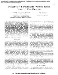
hardware design and energy consumption results can be found in [10]. A. Design Objectives The network is able to support multi-hop tree topology so that a large area can be covered. For example, monitoring environmental noise of surrounding areas of open air rock concert, the network should cover several hundred square meters. In a network size this means that it has 2-3 clusters which each includes 3 to 6 noise sensors. Throughput should be high enough so that the loss of data does not affect the precision of long-term statistics. A global synchronization is necessary in order to produce timely correlated noise data. The sensors are able to measure the acoustic noise continuously for a long enough period, usually for a whole weekend, and the cost of sensor nodes must be minimized. The most challenging feature of this application is the collection of large amount of noise data (72 bytes every 5 seconds for every sensor node in network) from the whole network, and delivering that to the sink node in a very short communication window. When a sensor node is measuring the noise, it has to turn off the radio transceiver due to that 1) noise ADC (Analog-to-Digital Conversion) sampling can not be interrupted, 2) radio activities are the source of significant interference to the sampling circuits. This leaves only a short time for all the sensor nodes to send and receive. Our first design was to let the sensor nodes near the SINK relay data for the remote sensors. Soon we found that it had a severe scaling problem when the number of sensors grows. In order to alleviate the bursty traffic, relay nodes are introduced for the remote sensors. Thus our target WSN contains a SINK node, a set of relay nodes, and a set of noise sensor nodes. The network topology is a multi-hop tree with SINK as the root of the tree. The sensor nodes can be deployed at any arbitrary location in the area concerned. An example application of such a network is shown in Figure 1. The relay nodes take care of relaying sensor packets to the sink. B. Platform Selection We choose IEEE 802.15.4 standard [11] compatible modules as our design platform for the following reasons: 1) We had already integrated (microcontroller + RF) modules, with the cross-layer architecture CiNet[12] implemented, which helped reducing the node size and the power consumption as well as the load on software development. 2) IEEE 802.15.4 is the de facto standard for WSN. This guarantees the portability and continuity of the project. 3) A sophisticated CSMA/CA MAC protocol eases the design of upper layer protocols. 4) IEEE 802.15.4 offers radio link statistics in terms of Receive Signal Strength Indication (RSSI) or Link

281

SENSORCOMM 2011 : The Fifth International Conference on Sensor Technologies and Applications

LAN/WAN

Cinet

Noise Measurement Sensor Network

Database/ HTTP server

Sensor node

Cross−layer

Application SYNC2SINK

Legends

Protocol Stack

Sink node

Power Saving

Management

Topology Synchro− Control nization

Relay node MAC(802.15.4)

Sensor node

Radio (CC2420)

Figure 1.

Noise measurement WSN example Figure 2.

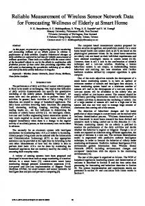
Quality Indication (LQI). This helps to implement a high throughput link-state routing protocol. In practice, two platforms are included in our development: one is a microcontroller-RF separated solution (ATmega128+CC2420) and the second is an integrated solution (Jennic JN5148). They work seamlessly in our testbed network. C. Networking and Synchronization We developed an integrated synchronization and routing protocol denoted as SYNC2SINK[13] to achieve our objectives. The SYNC2SINK protocol enables the nodes to establish and maintain a route to the sink using the information contained in synchronization frames. SYNC2SINK is built on the CiNet protocol stack[12], which is a crosslayer architecture in which time, radio link state, battery and topology information are shared by sensing, packet transmission and reception, and route table maintenance. The architecture of CiNet can be seen in Figure 2 In the SYNC2SINK protocol a node works periodically in 4 phases: synchronization phase, sensing phase, data communication phase, and optional sleep phase for energy saving. In this particular application the noise measurement has to be done continuously so that the sleep phase is removed. Thus the target network works periodically for synchronization, sensing, and data communications, denoted as Tsyn , Tsen , and Tcom respectively. However, note that during Tsen the radio part of the sensor nodes must be turned off due to the uninterruptability of noise sampling and interference reduction. Because the sensed data must be time-stamped, the SINK is synchronized by a server. The sensing phase is started synchronously right after the synchronization phase. The timeline activity of the network is shown in Figure 3.

Copyright (c) IARIA, 2011.

ISBN: 978-1-61208-144-1

System and node architecture T

Tsyn

Tsen

Tcom

Send to database server via GPRS Sink

Network nodes

Sampling ADC, constructing DATA frame

Round i

Figure 3.

Time Round i + 1

Timeline of the network operations

The SINK broadcasts SYNC frames periodically, with the period denoted as T. The frame size is 128 bytes in IEEE 802.15.4 networks. A current data frame can fit maximum of 4.5 second of noise data. Due to that, a 5 seconds sync period is chosen of which sensing phase is 4.5 seconds and 0.5 seconds is transmission phase. The broadcasting of SYNC has four functions: 1) let the whole network become synchronized, 2) let the relay nodes establish a route back to SINK, and 3) let the sensor nodes select the best relay node. The SYNC frame structure is shown in Figure 4(a) it has a length of 16 bytes, and function of its fields is given in Table I. More detailed function of the fields is illustrated in the following section. Correspondingly, in each synchronization period a sensor node sends a DATA frame back to the SINK. The length of the DATA frame is variable and the structure of DATA frame can be seen in Figure 4(b), in which the SeqNo field and GlobalTime is copied from the latest SYNC, SrcAddr and PredAddr are the addresses of the sending node and its predecessor, respectively. This address couple is used by the SINK to figure out the network topology. A relay/sensor node must be synchronized by the a SYNC frame, as it is not possible to relay or deliver any data if no

282

SENSORCOMM 2011 : The Fifth International Conference on Sensor Technologies and Applications

Power−on

Table I SYNC Field(octet) Type (1) SeqNo (1)

Symbol — si

SINKAddr (2)

Asink

PredAddr (2) MaxTTL (1/2)

Apred T T L∗

TTL (1/2)

TTL

Bat (1/2)

B

ST(1/2) RSSI (1) Thpt (1)

— Qrssi Ψ

Cmd (1) CmdData (1) GlobalTime (4)

(1)

(1)

Type SeqNo

Description Indicate that this is a SYNC frame Sequence number that increments every cycle Network address of the originating sink node (short IEEE 802.15.4 MAC address) the predecessor of the sending node The upper nibble is the initial value of TTL and kept constant during the broadcasting; the lower nibble is set by SINK as T T L∗ and decremented by each node, so that the nodes can calculate the hop count to the SINK. The upper nibble, indicating the battery residual of the sending node. Indicate the sending node type. Indicate the link quality Downlink throughput, basically a statistics of SYNC frame reception rate, can be used to estimate the uplink performance. Network command given out by SINK. Network command parameter Global time in seconds

— — Tg

(2)

(2)

(1)

SINKAddr

PredAddr

TTL

(1)

(1)

(1)

RSSI

Thpt

(1)

(1)

(4)

CMD Cmdbyte

GlobalTime

SenderType

Battery

(a) SYNC frame structure (1) Type

(1) SeqNo

(2)

(2)

SrcAddr

PredAddr

(1)

(1)

(4)

Length PredRSSI Timestamp

(1)

(1)

Ind

DataLen

(Length) Sensor DATA

(b) DATA frame structure Figure 4.

SYNC and DATA frame structure

route is established. The relay/sensor node must follow a strategy where: 1) When powered up, a node sets the radio module to receive the mode and starts waiting for a SYNC frame for a SYNC-hunting time tsh when tsh ≥ T. 2) If the SYNC frame is received within tsh time, the node takes the information from the SYNC to the route entry which contains 1) SINKADDR, 2) seqno, 3) predecessor addr, 4) Hop-count to SINK, 5) Link Quality (RSSI); then rebroadcasts the SYNC after the decrementing TTL field. The node is then running in Synchronized mode. 3) If no SYNC frame has been received within tsh , the node turns off the radio and sleeps for a random backoff time tbk . When tbk expires, the node goes back to Step 1. Such an operation will prevent the node from spending unnecessary energy in SYNC-hunting mode. 4) If the node is in synchronized mode and the next m consecutive SYNC frames are missed, the node will

Copyright (c) IARIA, 2011.

SYNC is received

FRAME STRUCTURE

ISBN: 978-1-61208-144-1

SYNC hunting

Synchronized m consecutive SYNC are missed

sleep over

no SYNC received

Random sleep Next SYNC is received

Figure 5.

The state-transition diagram of SYNC2SINK

B

good link

good link

A

C

poor link (a)

Figure 6.

poor link A

poor link

B

good link C

(b)

Problem of simple first-SYNC-routing

turn back to sync-hunting mode. The state-transition diagram of the nodes is shown in Figure 5. D. Link-State Routing In our first design, the relay/sensor nodes establish the route path to the SINK by the taking parameters of the first received SYNC frame (i.e., a greedy algorithm). We found that the DATA frame Packet Receive Ratio (PRR) to SINK was very poor. This is due to the fact that radio links established by the strategy may be poor, because the first arrival SYNC usually comes from a node over the maximum distance. As shown in Figure 6(a), a better choice might be to have a two-hop route from node C to node A, using node B in the middle as a relay, even though C hears SYNC from the A node first. In order to overcome this problem, we adopt a linkstate routing protocol (Power-Aware Routing - PAR[14]). We utilize RSSI, which is a default IEEE802.15.4 MAC layer information. Upon the reception of a SYNC frame, the receiving node can choose a more favourable predecessor as a relay to SINK. According to [15], [16] and a number of related works, an RSSI>-75dBm or equivalently LQI>90 indicates a PRR≥90% over a single link. The logic of PAR can be depicted as: if a node has received a SYNC frame with new SeqN o, it takes the sender of this SYNC as predecessor and mark the RSSI in the route entry; If a node has received a SYNC frame with the same SeqN o, it compares the RSSI with the previous one in the route entry. If 1) the new SYNC RSSI is within the range between a lower limit QL and a higher limit QH , 2) the old one is less than QL , 3) the hop count of the new one is no more than the old one plus 2, and 4) the sending node’s predecessor is not the receiving node; the receiving node will replace the route entry by the new SYNC’s information. If all the SYNC frames that come to this node have RSSI lower than the threshold, the node will simply use the first

283

SENSORCOMM 2011 : The Fifth International Conference on Sensor Technologies and Applications

Function processSYNCframe(Q∗rssi ,TxID)

T

T T L∗ and T T L

return: boolean(TRUE: rebroadcast SYNC, FALSE: do nothing)

Tsyn

B and ST

Legend:

C

A DATA frame

SINK

Start

Type SeqNo Asink Tx Mode

Apred TTL = TTL − 1

Qrssi P si

CMD RSV

R1

Rx Mode

$T_G$

Hop count to SINK H = T T L∗ − T T L

Sleep Mode R2

Qnew = min(Q∗rssi , Qrssi )

R3

YES

New SeqNo?

sensors

NO

UpdateRouteEntry by ModifySYNCframe by

and NO

t0

t0

(T T L, H, Qnew , Apred )

H < Re.H + 2

Figure 8.

Inter-layer scheduling

(T T L, Qrssi , Apred )

Q∗rssi ∈ (QL , QH ) and

TxID 6= Apred and

Return TRUE

Re.Qrssi ∈ / (QL , QH ) YES UpdateRouteEntry by

(T T L, H, Qnew , Apred )

Return FALSE

Figure 7. Flowchart of SYNC frame processing (Re.x represent the parameter stored in Route Entry)

one. Here we set a higher limit QH in order to prevent too short hops. As an example illustrated in Figure 6(b), both B and C have a poor link to A; however, when B receives a rebroadcast SYNC frame from C with a good RSSI, it shall not replace A by C as its predecessor. The flowchart about the processing of a SYNC frame is given in Figure 7. The result of adopting the link-state routing can be seen in Section IV. IV. R ESULTS AND A NALYSIS Before setting up a testbed network, important parameters such as Tcom , Tsyn must be determined. These parameters are tightly bounded by the hardware properties such as clock oscillator precision, physical and MAC layer features of IEEE 802.15.4 such as CSMA/CA slot time and contention window. As mentioned in Section III, noise sampling must be as continuous as possible —therefore both Tsyn and Tcom shall be kept small. A. SYNC Phase Time Tsyn A broadcast frame in IEEE 802.15.4 MAC does not require acknowledgement. According to the analysis in [17], the upper-limit time of broadcasting a SYNC takes tbc =randombackoff([0, 23 − 1] × 320µs)+ dataframeduration(352µs)+ turnroundtime(192µs).

Copyright (c) IARIA, 2011.

ISBN: 978-1-61208-144-1

This gives that the maximum tbc = 2784µs. Thus the phase time for synchronization is Tsyn = TTL∗ × tbc × D

(1)

where D is the node density in terms of the node number that can hear each other in a given area. This analysis does not consider the processing delay in each rebroadcasting node, which is actually a variable due to the task scheduling features of the running operating system. However, the processing of a broadcast message should be set as the highest priority task because this type of messages usually contains network management/control information, thus resulting in very short delay comparing to Tsyn . B. Transmission Scheduling At the end of every cycle, each sensor node generates a DATA frame and sends it out. If we try to deliver all the data frames to the SINK within a small time slot, it will create a burst of radio traffic and PRR can not be optimistic. In order to mitigate the problem, we set up both inter-layer and intra-layer transmission schedules. Here “layer” means the hop count to the SINK. Inter-layer scheduling is based on hop count to the SINK, denoted as H. Each relay node schedules the radio transceiver into the transmitting mode by ttx (H) = C · (T T L∗ − H) + T0 = C · T T L + T0

(2)

where C is the scaling constant, and T0 is the cycle starting time. Figure 8 shows an example. By this scheduling the remote nodes start the forwarding of DATA frames earlier than those closer to the SINK, and data frames are accumulated to the SINK in C × T T L∗ time. Intra-layer scheduling is done by the order of rebroadcasting SYNC frame. Since a SYNC frame can be heard by all the nodes in radio range, each node marks the sequence of its own broadcasting, and schedules the transmission by tc (S) = ttx (H) + (S

mod D′ ) · C ′

(3)

284

SENSORCOMM 2011 : The Fifth International Conference on Sensor Technologies and Applications

ti

Layer H + 1 C S=0

T

C

B S=0 A S=0

B S=1 A S=0

S=2

SYNC Frame

A S=0

(c) B wins the CSMA/CA, SB = 1

Sink time

SYNC Frame

Time Adjustment between Server PC and the SINK Table II T ESTBED NETWORK SETTINGS

(d) C is the last one, SC = 2

Cycle time T Data frames k per cycle Data frame length Tcom , Tsen Node time precision Inter-layer Delay Constant C Run time of each senario QH (LQI) QL (LQI)

Intra-layer scheduling among nodes A, B, and C

where ttx (H) is obtained from (2), C ′ is a scaling factor, D′ is predefined node density, and S is the sequential number of rebroadcasting SYNC frame in the same layer. An example of determining S is illustrated in Figure 9. A modulus operation bewteen S and D mitigates the scaling problem. However, if the node density is too high in some areas, multiple nodes will get the same tc and in this case they will rely on IEEE802.15.4 CSMA/CA to avoid collisions. C. Server-Sink Synchronization The SINK acts simply as a passthrough gateway between the WSN and a webserver which manages the sensor data in the SQL database. Therefore the measurement must follow the server time so that sensor data can be correctly stored and displayed. The connection between the server and the sink is either a direct RS-232 link or a GPRS channel. In order to synchronize with the server time, a fine adjustment is implemented between the SINK and the server as illustrated in the follow. Right after a SYNC frame has been sent out, the SINK immediately sends a polling message to the server. After the reception of the polling message, the server records the time when the message arrives, and compares it with the time of the previous arrival, denoted as δi = ti+1 − ti − T, and immeadiately sends δi in a reply message, as shown in Figure 10. The SINK adjusts its next SYNC broadcasting time by Ti+1 = Ti + T + δi . This adjustment will force the SYNC broadcasting to follow the server time. This simple time adjustment worked fine in our testbed. We tested the algorithm for nearly 1 day and the synchronization was maintained well (with mean δ only 0.0767ms).

5 sec. 1 80 bytes 1/4 sec. 0.001 sec. 0.15 sec. 7200 sec. or over night 150 varying

the LQI threshold, to obtain an optimal LQI threshold. In the third scenario, single-hop capacity was tested. The last two scenarios were designed to verify dynamic routing and multi-hop communication performance, respectively. More detailed protocol parameter settings are given in Table II for all the scenarios. We first put five noise sensor nodes in a coffee room to exam the synchronization performance. Figure 11 shows the time-line of the measurement results, and it can be seen that they are time-correlated. Then we set up a test network which has nine relay nodes

90 node 1, mean=66.16dBA node 2, mean=63.97dBA node 3, mean=65.69dBA node 4, mean=65.08dBA node 5, mean=66.50dBA

80

Sound level (dB)

Figure 9.

Ti+1 = Ti + δ

Figure 10.

B S=1

A S=0

poll

Ti

RF

S=2 C

Reply(δ)

poll

(a) SYNC rebroadcast from layer H to layer H + 1 (b) A wins the CSMA/CA, SA = 0

B S=1

Server time

Reply(δ)

Sink

C

ti+1

Server

S=1

UART via GPRS

Layer H

70

60

50

40

D. Test Settings We designed 5 scenarios to test different aspects of our communication protocol. In the first scenario, we examined our synchronization performance. In the second scenario, we tested the link-state routing performance by varying

Copyright (c) IARIA, 2011.

ISBN: 978-1-61208-144-1

30

3.254

3.256

Figure 11.

3.258

3.26

3.262 time (s)

3.264

3.266

3.268 x 10

4

Measurement result of 5 nodes in a coffee room

285

3.

SENSORCOMM 2011 : The Fifth International Conference on Sensor Technologies and Applications

95

0x5503/0.927 0x5505/0.979 0x5504/0.969

0x5007/0.979

Average of all nodes 0x5006/0.975

90

0x5501/0.952

90.2%

96.4%

99.8% 0x5001/0.983 94.9%

Packet Delivery Ratio (%)

85

93.3% 0x5002/0.971

Relay(0x5506) 0x5008/0.973

92.9%

80

91.9%

98.2%

99.8%

75

0x5003/0.977

90.3%

99.8%

0x5009/0.975

88.0% 74.3%

100%

0x5005/0.971

0x500b/0.975 99.6%

70

99.8% 0x500a/0.977

65

0x5004/0.975

100% 0x5502/0.889

60 SINK(0x6666)

55

0

Figure 12. routing

20

40 60 80 LQI threshold in link−state routing

100

120

Figure 13. The 2-hop scenario setup and results. A solid line means that the link is used primarily. A dotted link means the link is occasionally used. The number associated to node is the node address.

Packet receive ratio at different LQI settings in Link-state (0x8888) SINK

and one SINK at 4th floor of our laboratory building. In each cycle, a relay node produces one data frame and sends it back to the SINK. Figure 12 shows the link-state routing performance with different LQI thresholds. Note that LQIth =0 (or RSSI=128dBm) indicates a non-Link-State routing protocol. It can be seen that at LQIth =90 (or RSSI=-75dBm) the PRR hits the maximum value in the multi-hop scenario, which improves PRR by 10% compared with that of LQIth =0. A low LQI threshold results in that the network has smaller number of hops from the sink to the most remote nodes, but the radio link goodput is poor due to the long distance of the hops. On the other hand, a high LQI threshold gives a good radio link performance, but a remote data packet has to be relayed by more nodes back to the SINK, and it also aggravates the hidden node problem [18]. The third test was for single-hop capacity. We set up a number of sensor nodes as the first layer from a SINK. It can be seen that using intra-layer scheduling, one SINK can serve up to 14 sensor nodes with an average PRR greater than 96%. Table III shows the results of setting 12, 13, and 14 nodes respectively. Table III S INGLE - HOP PACKET D ELIVERY P ERFORMANCE Node No. 12 13 14

P RRmin 0.9870 0.9739 0.9301

P RRmax 0.9978 0.9942 0.9892

Mean 0.9916 0.9868 0.9659

Our next scenario was a two-hop setup with 1 relay and 16 sensors. This setup was meant to exam the dynamic routing performance. The result given in Figure 13 shows how well the dynamic link-state routing performs. The second column

Copyright (c) IARIA, 2011.

ISBN: 978-1-61208-144-1

R1 (0x5501)

R2 (0x5502)

R3 (0x5503)

99.9 98.8

100

98.1

99.9

98.7

100

100 0x5006

0x5003 0x5005 0x5001

0x5002

0x5004

100

0x5009 0x5008

0x5007

Figure 14. The 4-hop scenario setup and link usages. A solid line means that link is used primarily (usage in %). A dotted line means the link is occasionally used. The number associated to node is the node address.

of Table IV shows the PRR results. A node mostly sends data to its closest SINK/relay, and in case of link fluctuation, almost all of them have tried the alternative route. The last scenario was a 4-hop setup with 3 relays and 9 sensors. This setup was meant to exam the scalablity of routing protocol. The setup scenario is shown in Figure 14. PRR results are in the third column of Table IV. Results are good and it shows that scheduling works. V. C ONCLUSION In this paper we report the design and implementation of a protocol suite for a WSN application which measures the instantaneous environmental acoustic noise in a given area. The protocol features synchronization, link-state routing, and can be deployed/retrieved quickly. A good packet delivery ratio is achieved by carefully adjusting the timing and linkstate parameters. The most significant unique feature of our design is the support of multi-hop communications, which makes large-scale noise measurement possible. This feature has not been seen in any peer solution.

286

SENSORCOMM 2011 : The Fifth International Conference on Sensor Technologies and Applications

Table IV 2- HOP AND 4- HOP L INK - STATE P ERFORMANCE Node addr 5506 5501 5502 5503 5001 5002 5003 5004 5005 5006 5007 5008 5009 500a 500b 5501 5502 5503 5504 5505

PRR 2-hop 0.957 0.983 0.971 0.977 0.975 0.971 0.975 0.979 0.973 0.975 0.977 0.975 0.952 0.889 0.927 0.969 0.979

PRR 4-hop 0.984 0.969 0.957 0.978 0.975 0.977 0.966 0.967 0.965 0.947 0.956 0.956 -

R EFERENCES

[8] SoundEar. Soundear pro noise measuring system. [Online]. Available: http://www.soundear.com/images/stories/ produktblade/SoundEarPRO PP UK.pdf [Accessed: 201105-20] [9] APL Systems. (2011, 05) Apl aures. APL Systems. [Online]. Available: http://www.apl.fi/index.php?page id=4277 [Accessed: 2011-05-20] [10] I. Hakala, I. Kivela, J. Ihalainen, J. Luomala, and C. Gao, “Design of Low-Cost Noise Measurement Sensor Network: Sensor Function Design,” in Proc. of The First International Conference on Sensor Device Technologies and Applications (SENSORDEVICES 2010), July 2010. [11] IEEE standard Part 15.4: Wireless Medium Access Control (MAC) and Physical Layer (PHY) Specifications for Low-Rate Wireless Personal Area Networks (LR-WPANs), IEEE Std. [12] I. Hakala and M. Tikkakoski, “From vertical to horizontal architecture: a cross-layer implementation in a sensor network node,” in InterSense ’06: Proceedings of the first international conference on Integrated internet ad hoc and sensor networks. New York, NY, USA: ACM, 2006, p. 6.

[1] B. Raman and K. Chebrolu, “Censor networks: a critique of ”sensor networks” from a systems perspective,” SIGCOMM Comput. Commun. Rev., vol. 38, no. 3, pp. 75–78, 2008.

[13] I. Hakala and C. Gao, “Sync2sink: combining synchronization and routing for ieee 802.15.4-based sensor networks,” in Technical Report, 2009.

[2] European Commission. (1996) Green paper on future noise policy. com (96) 540 final, november 1996. Official Journal of the European Communities. [Online]. Available: http: //ec.europa.eu/environment/noise/pdf/com 96 540.pdf [Accessed: 2011-05-30]

[14] C. Gao and R. J¨antti, “A reactive power-aware on-demand routing protocols for wireless ad hoc networks,” in Proc. IEEE VTC 2004 Spring, Milano, Italy, May 2004.

[3] WHO. Occupational and community noise. World Health Organization. [Online]. Available: http://www.who.int/peh/Occupational health/OCHweb/ OSHpages/OSHDocuments/Factsheets/noise.pdf [Accessed: 2011-05-20] [4] European Commission. (2002, 07) Directive 2002/49/ec of the european parliament and of the council of 25 june 2002 relating to the assessment and management of environmental noise. Official Journal of the European Communities. [Online]. Available: http://eur-lex.europa.eu/LexUriServ/ LexUriServ.do?uri=OJ:L:2002:189:0012:0025:EN:PDF [Accessed: 2011-05-30] [5] S. Santini, B. Ostermaier, and A. Vitaletti, “First experiences using wireless sensor networks for noise pollution monitoring,” in REALWSN ’08: Proceedings of the workshop on Realworld wireless sensor networks. New York, NY, USA: ACM, 2008, pp. 61–65.

[15] K. Srinivasan and P. Levis, “RSSI is Under-Appreciated,” in EmNetS, 2006, 2006. [16] R. Maheshwari, S. Jain, and S. R. Das, “A measurement study of interference modeling and scheduling in low-power wireless networks,” in SenSys ’08: Proceedings of the 6th ACM conference on Embedded network sensor systems. New York, NY, USA: ACM, 2008, pp. 141–154. [17] N. Boughanmi, Y. Song, and E. Rondeau, “Wireless networked control system using ieee 802.15.4 with gts,” in in proc. 2nd Junior Researcher Workshop on Real-time Computing (JRWRTC) 2008, 2008. [18] A. Bachir, D. Barthel, M. Heusse, and A. Duda, “Hidden nodes avoidance in wireless sensor networks,” in Wireless Networks, Communications and Mobile Computing, 2005 International Conference on, vol. 1, June 2005, pp. 612–617 vol.1.

[6] L. Filipponi, S. Santini, and A. Vitaletti, “Data collection in wireless sensor networks for noise pollution monitoring,” in Proceedings of the 4th IEEE/ACM International Conference on Distributed Computing in Sensor Systems (DCOSS’08), Santorini Island, Greece, Jun. 2008. [7] Metravib.com. Wed007 noise dosimeter exposimeter. Website. [Online]. Available: http://www.01db-metravib.com/ environment.13/products.16/wed007.460/?L=1 [Accessed: 2011-05-20]

Copyright (c) IARIA, 2011.

ISBN: 978-1-61208-144-1

287