Design of Low-Cost Noise Measurement Sensor Network - CiteSeerX

Design of Low-Cost Noise Measurement Sensor Network: Sensor Function Design Ismo Hakala, Ilkka Kivel¨a, Jukka Ihalainen, Jari Luomala, Chao Gao University Of Jyv¨askyl¨a Kokkola University Consortium Chydenius P.O.Box 567, FI-67701, Kokkola, Finland {ismo.hakala, ilkka.kivela, jukka.ihalainen, jari.luomala, chao.gao}@chydenius.fi Abstract—In this paper, we report the sensor function design and implementation of a wireless sensor network application for measuring environmental acoustic noise. The system is built on ATmega128 and CC2420 platform. The protocol stack is based on CiNet stack with a global synchronization scheme and supports multi-hop communications. Strict filtering function specified by ITU-R 468 (namely A-weighting) is followed. Both the indoor and outdoor test results were compared with standard sound level meters (CESVA SC-20c and Pulsar94) and showed a less than ±2dB error in both short-term and longterm measurement. Power consumption has been measured that a single AA-type battery can sustain the application. Comparing to the traditional noise measurement method, our wireless sensor network solution is much lower in cost, able to offer real-time data with sensed data timely coherent, and requests least attention after deployment. Keywords-sensor node design; noise measurement; environment monitoring

I. I NTRODUCTION AND M OTIVATION In WSN (Wireless Sensor Network) development, sensor node design is never a trivial task due to the small size, low-cost, resource-limit nature of WSN applications. A requirement of measuring acoustic noise in both industrial and residential environments is present in Ostrobothnia area of Western Finland. In such a measurement system, a number of wireless sensor nodes must be scattered into a concerned area. Each node measures the noise level at its location and the data is collected by a sink node, which forwards the data to a web-based database. The network should be able to cover a large area such as a university campus, an industrial park, or a residential block. In many countries the environmental noise has been regarded as a critical metric of working and living comfort. However, traditional way of conducting noise measurement exhibits great inconvenience: A test technician needs to carry a sound level meter to a measuring location and set the meter up for a specific measurement duration, which is usually several hours, and repeat this procedure for all the measuring points. The disadvantages of this method are obvious: 1) commercial sound meters are expensive, making large scale measurement very costly, 2) point-by-point measurement makes the result incoherent in time, 3) due to the lack of communication facility, the measured result is not available in real-time, and 4) the sound meter has to be fully attended,

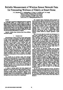
which increases the work load. These give the motivation of our WSN design. The goal of sensor node design is to minimize the necessity of peripheral components of a given microcontroller chip so that the cost of sensor is minimized. The target WSN consists of a sink and a set of noise sensor nodes. The network topology is therefore a multihop tree as the sink node the root of the tree. This network can be deployed in both indoor and outdoor environments. The sensor nodes should keep measuring the noise level for e.g., a whole day [1]. Comparing to the traditional method, our system has the following significant advantages: 1) cost reduction in both sensing devices and workload; 2) real-time, multi-point, coherent measurement; and 3) least attention. This WSN application has very special features because it demands excessive CPU power for data acquisition: the sensor nodes have to continuously sample the noise, thus leaving very short time for communication. The aim of this paper is to present the solution approaches to achieve accurate sensing and efficient communication for excessive data acquisition WSN applications. In order to accomplish multi-hop communications, we built our application on CiNet platform [2], which is a IEEE802.15.4-based platform using ATmega128 microcontroller with a cross-layer protocol stack containing efficient routing, topology management, and synchronization functions [3]. The block diagram of sensor node architecture can be seen in Figure 1. This document mainly covers the sensor function design. The networking and data communication issues are briefly illustrated in Section VI. However, they are thoroughly presented in our technical report, which will be published later. The rest of this document is organized as follows: A brief survey of related work is given in Section II; Background of sound level and its calculation is illustrated in Section III; Section IV covers the hardware design; Section V covers the software design and device calibration; Section VII shows the results of measurement and the comparison to a referencing device; Finally, Section VIII summarizes the design. II. R ELATED W ORK The work carried in [4] is probably the closest one comparing to our project. In their project, Tmote Sky

LAN/WAN

Cinet

Database/ HTTP server

Sensor node

Cross−layer

Application SYNC2SINK Protocol Stack

Power Saving

Management

Topology Synchro− Control nization

MAC(802.15.4) Radio (CC2420)

Figure 1.

System and node architecture

platform [5] were used, and the sensors were deployed to measure road traffic noise. Furthermore, from the measured data it is able to count the number and type of vehicles. The authors asserted that large-scale noise measurement using WSN solution is possible. However, the precision of measurement was not mentioned, the calibration of nodes was an open issue, and the sampling rate of sensor was set at 8kHz due to the CPU/ADC limit. In [6], the authors claimed that an environment monitoring system must have autonomy, reliability, robustness, and flexibility characteristics. They implemented a testbed network based on 8MHz TinyNode platform with 868MHz XE1025 transceiver to monitor the hydrological model of Alps area in Swissland. The authors in [7] proposed a WSN framework for environmental monitoring. The authors introduced a Sensorbased, Distributed Signal Processing (SbDSP) infrastructure to handle the acoustic data in a distributed way. However, detailed implementation was not included in the paper. In [8], a WSN was developed for coal mine monitoring to (1) rapidly detect the collapse area and report to the sink node, (2) to maintain the system integrity when the sensor network structure is altered, and (3) provide a sound and robust mechanism for efficiently handling queries over the sensor network under unstable circumstances. The system was built on Mica2 motes platform and a prototype has been deployed to D.L. coal mine in China. There is a bluetooth-based solution for noise measurement available in market [9]. In this solution, a bluetooth piconet, which supports maximum 5 noise nodes, can be deployed. It does not support multi-hop communication and therefore the application is limited within a small scale.

III. BACKGROUND : S OUND L EVEL Sound is a traveling wave, which is an oscillation of pressure transmitted through a solid, liquid, or gas, composed of frequencies within the range of hearing and of a level sufficiently strong to be heard, or the sensation stimulated in organs of hearing by such vibrations [10]. This wave energy can be picked up (i.e., heard) by the human ears. The human ears are very sensitive devices, which can hear sound power in a wide range of 12 to 13 decimal magnitudes [11]. Sound power level is thus defined as logarithm scale, denoted as decibels, and can be calculated by !   p2rms prms Lp = 10 log10 dB, (1) = 20 log 10 p2ref pref where prms and pref are RMS (Root Mean Square) sound pressure and reference sound pressure, respectively, and pref = 20µPa (RMS). The human ear is able to hear frequencies from 20 Hz to 20 kHz. However, it does not have a flat response to all the frequencies in the range, therefore in sound level measurement the sound signal is often frequency-weighted so that the measured level will match the ear-perceived level. Such a frequency weighting devices is also called weighting filter due to its frequency response feature. The IEC (International Electrotechnical Commission) has defined several weighting schemes, namely A, B, C, and D weighting. A-weighting is valid for relatively quiet sounds, which fits the application of our project. A-weighting filter is a frequency-select filter picking up the frequency range around 3-6 kHz, to which the human ear is most sensitive, while attenuating very high and very low frequencies to which the ear is insensitive. The corresponding transfer function of A-weighting filter is given according to [12] as 7.39705 × 109 · s4 . (s + 129.4)2 (s + 676.7)(s + 4636)(s + 76655)2 Figure 2 shows the frequency response of A-weighting filter, in comparison with B- and C-weighting filter curves. Sound level which is measured after A-weighting filter is also denoted as LA . The effective sound pressure is the RMS value of the instantaneous sound pressure over a given interval of time (a.k.a., time-averaging sound level). In general, it is called equivalent sound level over time T and denoted as LeqT . Three of these time-weightings have been standardized in IEC-61672(2003): ’S’ (T = 1 second) originally called Slow, ’F’ (T = 125 milliseconds) originally called Fast and ’I’ (T = 35 milliseconds) originally called Impulse. A general equation of LeqT for discrete system is denoted as ! N −1 1 X p2i , (2) LeqT = 10 log N i=0 p2ref HA (s) =

A. Signal Amplification and Dual Channel for Dynamic Range

1

10

0

Frequency Response (dB)

10

−1

10

−2

10

−3

10

B−weighting C−weighting Design A−weighting

−4

10

1

2

10

10

Figure 2.

3

4

10 Frequency (Hz)

10

A-weighting filter frequency response

PD4 GH MAX4465

A−Weighting

ADC

Mic MAX4524

GL MAX4465

Figure 3.

ATmega128L

Overall block diagram of noise measurement circuits

where N is the number of samples taken in time T . In our design, a set of digital and analog amplifications are introduced for a suitable ADC (Analog-to-Digital Converter) range. All these amplifications, together with pref , can be treated as a single constant and able to be retrieved by comparing the ADC readings with a standard calibrator.

IV. D ESIGN A PPROACH : H ARDWARE Research has shown that a long-term exposure to sound level over 85dB will cause hearing damage [13]. The average sound level of motorway traffic is 70dB and definitely regarded as an uncomfortable noise. Typical environmental or background noise level in residential areas ranges from 30dB to 80dB. Considering some measurement margins, this requires a dynamic range of 60dB more of measurement range. The focus of this chapter is to describe our hardware design that covers a dynamic range of 60+dB. The overall block diagram of sensor circuits is given in Figure 3. The sound pickup device is Monacor MCE-400 high-quality electret omnidirectional microphone cartridge [14]. The frequency range of MCE-400 fits well into Aweighting frequency curve.

As mentioned previously, one of the design objectives is to measure the noise level in a range of [30,90+]dB, which requires the data sampling and conversion system to cover a dynamic range of 60+dB. ATmega128 comes with a 10-bit build-in successive approximation ADC. 10-bit resolution can compensate a dynamic range of 20 log10 210 ≈ 60dB only, which does not meet the requirement. In order to solve the problem, we used two different preamplification gains to measure the sound levels in different ranges. As shown in Figure 3, two MAX4465 pre-amplifiers are in parallel arranged after the microphone. When the input level is low, the high-gain channel is selected; otherwise the low-gain channel is selected. A MAX4524 4-channel multiplexer is applied to select proper channel with the selection controlled by PD4 output pin of ATmega128. We here denote the two gains, GL , GH , respectively. In our design, GH = 390, GL = 10. Therefore, the dynamic range G2 is increased by 10 log10 GH2 = 31.82dB correspondently. L The sampling program starts from measuring the highgain channel input and keeps tracing the ADC input level. When a threshold is reached, PD4 is pulled low and the ADC input is switched to the low gain channel. Figure 4(a) is the oscilloscope snapshot of channel selection moment. It can be seen, that when the high-gain input gets saturated, PD4 is pulled down immediately and the low-gain input is selected. When the low-gain channel is selected, and the sound level goes below a threshold, the system will switch back to the high-gain, as shown in Figure 4(b). B. A-Weighting Filter According to the transfer function HA (s), the Aweighting filter can be approximated by a cascading of 3 high-pass plus 2 low-pass filters. The frequency response of such a filter is also plotted in Figure 2. Need to mention that theoretically such a filter can be implemented by software as a digital filter. However, a digital filter involves excessive floating point calculation which definitely surpasses the limit of 8-bit ATmega128. V. D ESIGN A PPROACH : S OFTWARE The software is designed to be able to perform both slow and fast measurements: the RMS power calculation is done every 125ms and 1s corresponding to F/S time-weightings in IEC 61672, respectively. A. 10-bit ADC setting The 10-bit ADC is set in differential channel mode at 33kHz sampling rate. Such a sampling rate has frequency response from 0 to 16.5kHz, which covers the range of A-weighting filter well, therefore most of sound power is

3.5

lected. Thus we can accept an instantaneous peak voltage to the reference of Vp|peak =1.5-Vn =Vn -1.0=0.25V. If we assume that the input sound wave is a sinusoidal for the first order approximation, the√RMS voltage of microphone input Vrms|mic =Vp|peak /GL / 2 = 17.7mV. The MCE-400 has sensitivity of 7.9mV/Pa, so 17.7mV corresponds to prms =2.24Pa sound pressure. Applying equation (1), it indicates that our system is able to measure sound level up to 100.98dB.

3 2.5

Channels + Offsets

2 1.5 1 0.5

B. Signal sampling and averaging

0 −0.5 High Gain input Low Gain input A−weigh Filter output MUX select

−1 −1.5

−0.8

−0.6

−0.4

−0.2

0 0.2 Time(s)

0.4

0.6

0.8

1

(a) Oscilloscope record of channel selection 3.5 High Gain input Low Gain input A−weigh Filter output MUX select

3

2.5

Channels + Offsets

2

1.5

1

0.5

The basic algorithm is to take samples and square each of them. At the end of each 1ms, if GH is being applied, in case the signal is too strong and clip has been observed, the MUX is turned into GL channel; if GL is being applied, in case the signal is weaker than a threshold ∆, the MUX is turned into GH . For every 125ms, an RMS average is calculated using equation (2). Algorithm 1 shows the algorithm in details, and Table I is the variable description for the algorithm. N1 Nm N1ms xi S1 Sm H c C ∆ RMS()

number of repeats in 1 second number of 1ms repeats in different modes (i.e., I/F/S) number of samples can be converted in 1ms instantaneous sample accumulative sum in 1 second accumulative sum in different modes threshold that a HIGHGAIN signal will clip the amplifier counter for the HIGHGAIN channel saturated threshold count that LOWGAIN channel should be selected threshold that LOWGAIN channel gives too small input RMS operation Table I VARIABLE D ESCRIPTION FOR A LGORITHM 1

0

−0.5

−1

−1.5 −0.02

C. Calibration 0

0.02

0.04

0.06

0.08 Time(s)

0.1

0.12

0.14

0.16

0.18

(b) Multiplexer selection pin activities Figure 4.

High/low gain channel selection

picked up by ADC. The conversion formula is given as [15]: ADC =

(Vp − Vn ) · GAIN · 512 , Vr

(3)

where Vn =1.25V is the negative input pin of ADC0, Vr =2.56V is the selected voltage reference, and GAIN =10 is the ADC’s internal gain. These three are constant values. Vp is the instantaneous voltage of positive input pin ADC1 fed by the A-weighting filter. According to (3), Vp must be in range of [1.0,1.5V] so that ADC output is in range of [-512, 511]. When Vp is at boundaries of range [1.0,1.5]V, the strongest sound pressure level is seen at the microphone input, and in this case the low-gain channel GL is se-

Calibration was done with CESVA SC-20c, which is a high performance Type I integrating-averaging sound level meter. SC-20c is able to send measurement data to a host PC via RS232 interface and the data can be stored in file for further analysis. The calibration acoustic source must be 1kHz sine wave. The ADCrms values are compared with CESVA measurement in range of [30,90] decibels and an empirical curve fitting equation is drawn as LpA = 8.1522 × ln(ADCrms ) + 32.7148(dB)

(4)

The calibration curve can be seen in Figure 5. VI. N ETWORKING & S YNCHRONIZATION The application requires multi-hop communication to send sensed data back to a sink, and a global synchronization is necessary to offer time-coherent noise information. We proposed a SYNC2SINK application-oriented protocol to accomplish the task. In this section we briefly describe SYNC2SINK mechanism. The details of networking and

T

Algorithm 1 Sound Level Calculation Algorithm Tsyn

for k=0 to N1 -1 do S1 = 0 for i=0 to Nm − 1 do Sm = 0, c = 0 for j=0 to N1ms − 1 do readADC to xi if xi > H then c++ end if Sm = Sm + x2i end for if HIGHGAIN then if c ≥ C then set LOWGAIN end if else Sm = Sm ∗ (GH /GL )2 if Sm < ∆ then set HIGHGAIN end if end if q 1 RMS(Sm )= N N Sm m 1ms end for record max(RMS(Sm )) and min(RMS(Sm )) S1 = S1 + RMS(Sm ) end for S1 mean(S1 ) = N 1 record mean(S1 ),max,min

Tcom Time

Sink

Network nodes

Sampling ADC, constructing DATA frame

Figure 6.

Time

Timeline of the network operations

receiving a copy of it, and sets the sender of that SYNC as its predecessor to sink, thus a passive route to Sink is established for every node throughout the network. Then the node goes into noise sampling phase which has been described in previous section. During this phase, the node turns off its radio transceiver so that the RF electromagnetic interference to the sampling circuits is eliminated. Each period is 5 seconds. The SYNC-broadcasting phase is no longer than 20ms and negligible. Sampling phase is 4 seconds and totally 32 125ms “Fast” RMS values are produced, leaving the last second for data communication. Each data frame contains 64 bytes RMS values (2 bytes for each 125ms) and some application layer overhead, resulting in a total of 96 bytes of payload are pushed to the IEEE 802.15.4 MAC layer.

100 LpA= (log(ADC) + 4.0135)/0.1227 (dB)

90

Sound level LpA (dB)

Tsen Send to database server via GPRS

VII. M EASUREMENT R ESULT & C OMPARISON

80

The final finish of our sensor node can be seen in Figure 7. The nodes are sealed by metal cover and waterproof material so that they can be deployed outside.

70

60

A. Power consumption 50 CESVA Fitting Curve

40

30

0

200

Figure 5.

400

600 ADC readings

800

1000

1200

Calibration and Curve Fitting

synchronization issues such as throughput control over multi-hop and clock skew control are presented in another document. SYNC2SINK is built on CiNet protocol stack [3] (Fig. 1). SYNC2SINK works periodically and each period consists of three phases: SYNC broadcasting, noise sampling, and data communication with durations denoted as Tsyn , Tsen , and Tcom respectively (Figure 6). Each period is started by the Sink node broadcasting a SYNC frame, which contains a monotonically increasing sequence number and the current time of the sink. Every node re-broadcasts the SYNC after

Instantaneous power consumption was tested by adding a 5.25Ω resistor next to the power supply. We measured the voltage over the resistor and calculated the current using Ohm’s rule. Similar method has been used in [16], [17]. In order to indicate the phases mentioned above, an output pin is triggered when there is a phase transition. In each period T the µC keeps reading ADC value and calculates the sound level. At the end of each period the radio module is turned on and a data frame is sent to the sink. When a sensor node is not scheduled to do radio communication, the radio module CC2420 is turned off to save energy. In this state the node consumes a constant, small amount of energy as shown in Figure 8(a). In general, the sensor nodes have sleep schedules. However, in this application the sensor nodes must keep sensing the noise thus no sleep mode is applied to µC. Nevertheless, we have observed less than 1mA current drain during the sleeping mode. We are interested in the real-time power consumption when the node is active and its radio is turned on. Totally five phases are needed to send a frame [18]:

Average = 26.90mA 60

50

Current (mA)

40

30

20

10 Power Consumption(mA) Time−indication pin 0 −200

0

200

400

600

800 1000 Time (ms*5)

1200

1400

1600

1800

(a) Power consumption in a sensing cycle (5sec) Average = 36.74mA 180

160

Figure 7.

t

t t

t

3

1

7

5

Final finish of the sensor node t

t

140

4

2

t

t

8

6

Current (mA)

120

1) Initialize radio module: the radio transceiver is turned on and the oscillator starts to oscillate. This phase takes a few milliseconds. 2) Frame formatting: a frame is copied to the radio buffer from µC. This phase duration varies, depending on the frame length. 3) Waiting RSSI: the radio module waits for a clearance of channel. This phase duration varies, depending on the channel situation. 4) Random backoff: IEEE 802.15.4 uses CSMA/CA media access control (MAC), so a random backoff will reduce the chance of collision. 5) Sending the frame: the frame is sent out. The duration is proportional to the frame length. The above phases can be seen in Figure 8(b). As the time transitions given by the time-indication-pin in Figure 8(b), the duration t2 − t1 is the radio initialization phase, which takes approximately 5ms. There is an impulse power consumption at the beginning of this time when the radio circuits oscillator starts to run. The second duration t3 − t2 indicates the local communication between ATmega128 and CC2420. In our test, a total of 37 bytes (including MAC header 9 bytes, IP header 20 bytes and payload 8 bytes) were copied to CC2420. SPI (Serial Peripheral Interface) was set at a bus clock rate 7.7MHz/16 so that 37 bytes will take 0.615ms to transmit. Together with SPI bus commands, we have observed approximately 1ms for this phase. The power consumption raises 5mA from a floor of 30mA during this time.

100

80

60

40

20 Power Consumption(mA) Time−indication pin 0

0

1

2

3

4

5 Time (ms)

6

7

8

9

(b) Power consumption during transmission Figure 8.

Power consumption

The third time is short. This is the time that CC2420 acknowledges to the µC that frame buffer is ready. The next duration t5 − t4 is the channel access time. CC2420 must find a valid RSSI (Received Signal Strength Indicator) before the attempting of transmission. During this time the radio module keeps listening to the channel so a few power peaks are observed. The duration t6 − t5 is the random back-off time of CSMA/CA, and t7 − t6 the frame transmitting time. During the transmission, the power consumption stays on a floor of 60mA. At last, during t8 − t7 the radio module is turned off. In average, sending a frame consumes 36.74mA in approximately 10ms, and the entire cycle average is

1,5 m

84

3 sensor nodes and Pulsar

Pulsar Node Avg Node Avg+δ Node Avg−δ

82

80

0,73 m

0,73 m

Sink node

Sound level (dB)

78

76

74

72

Figure 9.

70

Indoor test configuration

68

26.90mA. Consider a typical AA-type battery with capacity of 2500mAh [19], it can support the node for 2500 ∗ 3600/26.90 = 334570 seconds, which is nearly 93 hours, which satisfies the demand. Our field test experience has also proved this conclusion. Actually by network control/synchronization, the sensor nodes can be put into sleep mode, and wake up on demand. The network life time can be significantly increased by doing so.

66

C. Indoor accuracy test All the nodes have been tested with Pulsar94, a type II sound meter, in a noise-immune room. The test configuration can be seen in Figure 9. Nodes are tested and their microphone pick-up points are very close to the sound meter 1.5m away from the sound source. The sound source is traffic noise recorded at Colin McRae Gathering down the M6, Sandbach [20]. In order to reduce the error, we put Pulsar94 at different places in the array. The test duration is 30 minutes with each configuration 5 minutes. The result is shown in Figure 10. The result shows that our nodes give very close data to that of Pulsar94. The mean standard deviation among our nodes is 0.91dBA throughout the all test phases. D. Outdoor accuracy test The field test was conducted on an open ground close to a motorway. We arranged 5 noise nodes in a line perpendicular to the motorway with 10 meters separation one each other, and Node 1 being the closest to the road. We put Cesva SC20c together with each node and measured for 5 minutes. Because there is no synchronization between our network and SC-20c, we gave an impulse sound to mark the start of measurement. Figure 11 shows the results. We can see that our nodes have less than 2dB error for all the nodes.

50

100

150 Time (sec)

200

250

300

Figure 10. Indoor test results, presented as 3 nodes average together with Pulsar94. Deviations of nodes’ measurement are also given 100 Cesva Node 5 ( 1.18) Node 4 (−0.34) Node 3 (−0.83) Node 2 (−0.26) Node 1 (−0.57)

90

B. Node cost

80

Sound level (dB)

The cost of one sensor node is about 100 Euros. Comparing to the price of commercial sound meters in market, with the typical price for a class I sound meter 2000 Euros or more, this WSN application is very competitive.

0

70

60

50

40

200

400

600

800

1000

1200

1400

1600

Time (s)

Figure 11. Outdoor test – motorway noise (The measurement errors comparing to Cesva are given in the legend after each node, respectively)

VIII. C ONCLUSION & F UTURE W ORK In this paper, the design of wireless sensor node for environmental noise measurement is described. Technical challenges during the design are reported and corresponding solutions are explained. The comparison with standard Type 1 sound meter is made and the objective of design is achieved. The power consumption is small enough so that a typical AA-type battery can support the nodes for several days of measuring without sleep. ATmega128 build-in A/D converter is enough for environmental noise measurement thus the cost of hardware platform is minimized. The sensor node platform is built on ATmega128L with 4kB RAM, and its internal 10-bit ADC can operate a peak sampling rate of 33kHz. Both of these two resources have been pushed to their limits in our design. A better alternative should definitely have wider ADC range and more RAM. For this reason, we have decided our next development will

be continued on Jennic JN5139 platform, which has a 32-bit architecture, 16MHz clock, 12-bit ADC, and 96kB RAM. R EFERENCES [1] European Commission, “Directive 2002/49/ec of the european parliament and of the council of 25 june 2002 relating to the assessment and management of environmental noise,” Official Journal of the European Communities, 07 2002. [2] I. Hakala, M.Tikkakoski, and I. Kivel¨a, “Wireless sensor network in environmental monitoring - case foxhouse,” in Proceedings of the Second International Conference on Sensor Technologies and Applications (SENSORCOMM 2008), Cap Esterel, France, August 25-31 2008. [3] I. Hakala and M. Tikkakoski, “From vertical to horizontal architecture: a cross-layer implementation in a sensor network node,” in InterSense ’06: Proceedings of the first international conference on Integrated internet ad hoc and sensor networks. New York, NY, USA: ACM, 2006, p. 6. [4] S. Santini, B. Ostermaier, and A. Vitaletti, “First experiences using wireless sensor networks for noise pollution monitoring,” in REALWSN ’08: Proceedings of the workshop on Realworld wireless sensor networks. New York, NY, USA: ACM, 2008, pp. 61–65. [5] Moteiv Corporation. Now Sentilla (www.sentilla.com), TMote Sky Datasheet, Date retrieved: 20th of April 2010. [Online]. Available: http://sentilla.com/files/pdf/eol/ tmote-sky-datasheet.pdf [6] G. Barrenetxea, F. Ingelrest, G. Schaefer, and M. Vetterli, “Wireless Sensor Networks for Environmental Monitoring: The SensorScope Experience,” in The 20th IEEE International Zurich Seminar on Communications (IZS 2008), 2008, invited paper. [7] K. Lu, Y. Qian, D. Rodriguez, W. Rivera, and M. Rodriguez, “Wireless sensor networks for environmental monitoring applications: A design framework,” in Global Telecommunications Conference, 2007. GLOBECOM ’07. IEEE, Nov. 2007, pp. 1108–1112. [8] M. Li and Y. Liu, “Underground coal mine monitoring with wireless sensor networks,” ACM Trans. Sen. Netw., vol. 5, no. 2, pp. 1–29, 2009. [9] Metravib.com. Wed007 noise dosimeter exposimeter. Web page. Date retrieved: 20th of April 2010. [Online]. Available: http://www.01db-metravib.com/environment.13/ products.16/wed007.460/?L=1 [10] W. Morris, Ed., The American Heritage Dictionary of the English Language. Houghton Mifflin, 2000. [11] W. Boyes, Instrumentation Reference Book, 3rd ed. Butterworth-Heinemann, 2002. [12] IEC 61672 Ed.1.0, Electroacoustics - Sound level meters, Electroacoustics Std., 2003. [13] World Health Organization, “Occupational and community noise,” Web page. Date retrieved 20th of April 2010, 02 2001. [Online]. Available: http://www.who.int/mediacentre/ factsheets/fs258/en/

[14] Monacor International. Mce-400 high-quality electret microphone cartridge. Web page. Date retrieved: 20th of April 2010. [Online]. Available: http://www.monacor.de/ typo3/index.php?id=84&L=1&artid=5171&spr=EN&typ=full [15] ATmega128 8-bit AVR microcontroller datasheet, ATMEL Co.Ltd. [16] E. Erdogan, S. Ozev, and L. Collins, “Online snr detection for dynamic power management in wireless ad-hoc networks,” in Research in Microelectronics and Electronics, 22 2008-April 25 2008, pp. 225–228. [17] B. Hohlt, L. Doherty, and E. Brewer, “Flexible power scheduling for sensor networks,” in IPSN ’04: Proceedings of the 3rd international symposium on Information processing in sensor networks. New York, NY, USA: ACM, 2004, pp. 205–214. [18] TI CC2420 2.4GHz IEEE 802.15.4/ZigBee-ready Transceiver Datasheet, Texas Instruments.

RF

[19] A. L. P. Aroul, A. Manohar, D. Bhatia, and L. Estevez, “Power efficient multi-band contextual activity monitoring for assistive environments,” in PETRA ’08: Proceedings of the 1st international conference on PErvasive Technologies Related to Assistive Environments. New York, NY, USA: ACM, 2008, pp. 1–7. [20] Youtube video, “Colin mcrae gathering down the m6, sandbach,” Date retrieved: 20th of April 2010. [Online]. Available: http://www.youtube.com/watch?v=QXQEP37fxU