This tool is the observer coverability graph (OCG), and can be seen as an ... OCG represents both the set of reachable markings of a net system and the error of ...
Design of observers/controllers for discrete event systems using Petri nets Alessandro Giua, Carla Seatzu Department of Electrical and Electronic Engineering University of Cagliari, Italy {giua,seatzu}@diee.unica.edu
Abstract In this paper, that is an extended abstract of the talk presented at the Symposium on the Supervisory Control of Discrete Event Systems held in Paris in July 2001, we deal with the problem of estimating the marking of a Place/Transition net based on event observation. We assume that the net structure is known while the initial marking is only partially known and we give an algorithm to construct an observer that computes a marking estimate. The special structure of Petri nets allows us to use a simple linear algebraic formalism for estimate and error computation. The main advantage of this approach is that the proposed observer can also be used in a state feedback control loop.
Keywords: Petri nets, observability, marking estimation, supervisory control.
Published as: A. Giua, C. Seatzu, ”Design of observers/controllers for discrete event systems using Petri nets,” in Synthesis and Control of Discrete Event Systems, B. Caillaud, X. Xie, Ph. Darondeau and L. Lavagno (Eds.), pp. 167-182, Kluwer, 2001. 1
control γ
K
control γ
plant
L
controller w
legal words
controller M
legal states
word of events
state
(a)
(b)
control γ
L
control γ
plant
controller
L
w
model M=Mw
plant
controller µw Βw
M0
(c)
plant w
observer
(d)
Figure 1: Different control schemes. (a) Event–feedback. (b) State–feedback. (c) State–feedback with event observer and initial marking. (d) State–feedback with event observer and initial macromarking.
Introduction In this paper, that is an extended abstract of the talk presented at the Symposium on the Supervisory Control of Discrete Event Systems held in Paris in July 2001, we deal with the problem of estimating the marking of a Place/Transition net based on event observation and of controlling the net taking this estimate into account. The paper summarizes the main results obtained by the authors. For a more detailed discussion we refer to [7, 8, 9]. Motivation In the classical approach of Ramadge and Wonham [19] to the supervisory control of discrete event systems, the event-feedback control scheme shown in Figure 1.a is adopted. Here the plant spontaneously generates a word of events w. The supervisor observes the word of events generated and, given a set of legal words K, computes at each step a suitable control pattern γ to ensure that no illegal word be generated. Other authors have used a different state-feedback control scheme, shown in Figure 1.b. Here the supervisor observes the actual plant state M and, given a set of legal states L computes at each step a control pattern to ensure that no illegal state be reached. This scheme is particularly appealing when dealing with Petri net models of the plant [10], since the state of a net is given by an integer vector called marking (this explains the notation M used for the plant state in the figure) and linear algebraic techniques may be used to solve the control problem. A slightly different scheme is shown in Figure 1.c. Here the controller observes the word of events generated and, by means of an observer, it reconstructs the actual plant state M . The observer simply duplicates the plant model, and is driven by the observed events. If the structure (that is assumed to be deterministic) and the initial state M0 of the plant are known, the knowledge of the word generated is sufficient to reconstruct 2
the new state that each new firing yields. When the initial state is not completely specified a different control scheme may be used. In particular, we use Petri net models and assume that the initial marking M0 is known to belong to a “macromarking”, i.e., we know the token contents of subsets of places but not the exact token distribution. In this case we can use the control scheme shown in Figure 1.d. The estimation algorithm enables the computation of a marking estimate µw and an error bound Bw , and the control pattern γ is produced on the basis of the knowledge of µw and Bw . Proposed approach We assume that the net structure is known while the initial marking is unknown and we give an algorithm to construct an observer that computes a marking estimate that is a lower bound of the actual marking. The special structure of Petri nets allows us to use a simple linear algebraic formalism for estimate and error computation. The main advantage of this approach is that the proposed observer can also be used in a state feedback control loop. The error function between the actual marking and the estimate can be shown to be a monotonically non–increasing function of the observed word length. Observed words that lead to a null error are said to be complete. Complete observers are the discrete event counterpart of asymptotic observers for time–driven systems. Several observability properties may be defined. In particular, marking observability (MO) means that there exists at least one word that is complete, while strong marking observability (SMO) implies that all words can be completed in a finite number of steps into a complete word. All the considered properties can be proved either by the use of the observer coverability graph, i.e., the usual coverability graph augmented with a vector that keeps track of the estimation error, or by reducing them to other decision problems (e.g., home-space properties, marking reachability, existence of repetitive sequences) that can be checked using algorithms well known from the literature. Clearly, the use of marking estimates (as opposed to the exact knowledge of the actual marking of the plant) leads to a worse performance of the closed-loop system in the sense that to rule out the possibility that the plant enters a forbidden marking, the controller may prevent the firing of transitions whose firing is perfectly legal given the actual marking of the plant and this may lead to a deadlock. A general solution to the problem of recovering from an observer induced deadlock has been recently proposed by the authors in [2] and is based on an original linear characterization of the set of deadlock markings. Relevant literature Observability is a fundamental property that has received a lot of attention in the framework of time–driven systems, given the importance of reconstructing plant states that cannot be measured. Although less popular in the case of discrete–event systems, the issue of state estimation and of control under partial state observation has been discussed in the literature. For systems represented as finite automata, Ramadge [18] was the first to show how an observer could be designed for a partially observed system. The state estimation for finite automata models has also been ¨ studied by Caines et al. [3, 4] and Ozveren and Willsky [17], while Kumar et al. [11] defined observer based
3
dynamic controllers in the framework of supervisory predicate control problems. The main drawback of the above procedures is that at each step they require the exhaustive enumeration of the set of consistent states — i.e., the set of states in which the plant may be given the observed behaviour — that may reveal a highly complex task. On the contrary, the procedure we propose enables us to update the place marking estimation by simply determining the maximum among two integer numbers, and to completely define the new set of consistent markings as a convex set, only depending on the new marking estimate and the updated error bound. Very few works dealt with observability in Petri nets. As far as we know, the first one were [5, 7] where preliminary concepts discussed in this paper have been introduced. Meda et al. [15], Ram´ırez et al. [20] and Aguirre [1] used Interpreted Petri nets to model the system and the observer. In their approach both event firings and place markings can be (partially) observed and it is assumed that the token contents of all P-semiflows is initially known. The optimal choice of sensors to ensure that the plant is observable has also been discussed in [1]. The issue of controlling a plant with incomplete (state or event) measurements has also been discussed in the discrete event control literature. Zhang and Holloway [23] used a Controlled Petri Net model for forbidden state avoidance under partial event observation while the use of state-feedback control under partial state observation has been discussed by Li and Wonham [12, 13] and by Takai et al. [21]. In the work of these authors the partial observation is due to a static mask, that maps the plant state space into an observation space. The main focus was in finding necessary and sufficient conditions for the existence of “optimal” state feedback control laws given a mask (optimal means that the resulting closed-loop behavior is the same for the controller with mask and the controller with complete state observation). Unlike the above approach, the setting we dealt with assumes that the mask is induced by the computed estimate, and it changes as the plant evolves. Initially, when the estimate is crude, it is often the case that these restrictive “optimal” conditions are not verified. The control scheme we propose (see section 4) tries to make the best use of the available estimate to ensure the correct behaviour of the plant under control.
1
Background
In this section we recall the Petri net formalism used in this paper. For a more comprehensive introduction to Petri nets see [16]. A Place/Transition net (P/T net) is a structure N = (P, T, P re, P ost), where P is a set of m places; T is a set of n transitions; P re : P × T → N and P ost : P × T → N are the pre- and post-incidence functions that specify the arcs. The incidence matrix of the net is defined as C(p, t) = P ost(p, t) − P re(p, t). A marking is a vector M : P → N that assigns to each place of a P/T net a non-negative number of tokens, represented by black dots. A P/T system or net system hN, M0 i is a net N with an initial marking M0 . A transition t is enabled at M if M ≥ P re(·, t) (where P re(·, t) denotes the column of P re corresponding to transition t) and may fire yielding the marking M 0 = M + C(·, t). We write M [wi M 0 to denote that the enabled sequence (or word) of transitions w may fire at M yielding M 0 ; we use the notation M 0 = w(M ) and M = w−1 (M 0 ). Moreover, we denote w(M0 ) = Mw . Finally, we denote as w0 the sequence of null length. The set of all sequences firable in hN, M0 i is denoted L(N, M0 ) (this is also called the prefix-closed free language of the net). Let w = tα1 , tα2 , · · · , tαk be a sequence in L(N, M0 ). The sequence wi = tα1 , · · · , tαi with i ∈ N and i ≤ k 4
is a prefix of w of length i and we write wi 4 w. The prefix w0 of length zero corresponds to the empty sequence. A marking M is reachable in hN, M0 i iff there exists a firing sequence w such that M0 [wi M . The set of all markings reachable from M0 defines the reachability set of hN, M0 i and is denoted R(N, M0 ). Finally, we denote ~0m a m × 1 vector of zeros.
2
Marking estimation with event observation
The main focus of this section is that of presenting in detail the marking estimation procedure firstly proposed by one of the authors in [7]. We also recall some elementary properties of the estimate. Proofs are omitted here and can be found in [7, 8, 9]. In this paper we assume that partial information about the initial marking is available in the form of a macromarking. Definition 1 ([8]) Assume the set of places P can be written as the union of r+1 subsets P = P0 ∪P1 ∪· · ·∪Pr , where P0 ∩ Pj = ∅ for all j > 0, while any two sets Pj and Pj 0 may have a non null intersection if j, j 0 > 0. The characteristic vector of each set Pj is denoted ~vj , i.e., ~vj (p) = 1 if p ∈ Pj , else ~vj (p) = 0. The number of tokens contained in Pj (j > 0) is known to be bj , while the number of tokens in P0 is unknown. Let V = [~v1 , · · · , ~vr ] and ~b = [b1 , · · · , br ]. The macromarking V(V, ~b) is defined as the set {M ∈ Nn | V T · M = ~b}. We make the following assumptions. A1) The structure of the net N = (P, T, P re, P ost) is known, while the initial marking M0 is not. A2) The event occurrences (i.e., the transition firings) can be observed. A3) The initial marking M0 belongs to the macromarking V(V, ~b), i.e., it satisfies the equation V T · M0 = ~b. We also introduce the following notation. Definition 2 ([7]) After the word w has been observed we define the set M(w | V, ~b) of w–consistent markings as the set of all markings in which the system may be given the observed behaviour and the initial marking, i.e., the set M(w | V, ~b) = {M ∈ Nm | ∃M0 ∈ V(V, ~b), M0 [wiM }.
2.1
Main idea
The main idea of the estimation procedure is now sketched through a very simple example. Let us consider the net system in fig. 2, whose initial marking is that reported in fig. 2.a. We assume that the initial marking M0 belongs to the macromarking V(V, ~b) where V = [1 1 1]T and ~b = 3, i.e., we know that three tokens are contained in the net, but we do not know their exact location. Since our objective is that of providing a marking estimate that is always a lower bound of the actual marking of the net, we take as the initial estimate µw0 = [0 0 0]T , where w0 is the sequence of zero length (fig. 2.a’). As a consequence the initial bound is Bw = ~b = 3, i.e., three tokens still have to be detected. 0
5
p1
t2
p2
t3
t1
t2
p2
p3
(a’)
p2
p1
t3
t1
p3 p1
t3
t1
t2
(a)
p3 p1
p1
t2
p2
p3
t3
p3 p1
(b’)
p2
t1
(b)
t3
t1
t2
t2
(c) p2
t3
t1
p3
(c’)
Figure 2: A Petri net used in the illustrative example in section 2. Moreover, we define the set of w0 –consistent markings as M(w0 | V, ~b) = {M ∈ Nm | M (p1 ) + M (p2 ) + M (p3 ) ≤ 3}. This means that before any transition firing is observed, the actual marking of the net may be any vector within the macromarking V(V, ~b). Let transition t1 fires so that the observed word is now w1 = t1 and the net reaches the marking in fig. 2.b. Firstly we may update the previous estimate to µ0w1 = [0 0 1]T ; in fact, if transition t1 is enabled from the initial marking we can be sure that at least one token was initially contained in p3 . Moreover, after the firing of t1 the newly detected token is now contained in p1 , thus the new marking estimate is µw1 = [1 0 0]T (fig. 2.b’), and the new bound is Bw = 2. The set of w1 –consistent markings is M(w1 | V, ~b) = {M ∈ Nm | M ≥ 1
µw1 , V T · M = V T · µw1 + Bw1 }. Now, let transition t2 fires so that the observed word is w2 = t2 and the net reaches the marking in fig. 2.c. In this case no additional information is obtained because the fact that t2 is enabled implies that at least one token is contained in p1 , but this information was already known. The previous estimate is not updated, i.e., µ0w2 = µw1 , while the estimate after the firing of t2 is µw2 = [0 1 0]T (fig. 2.c’). Analogously, the bound does not change, i.e., Bw = Bw = 2 and the set of w2 –consistent markings is M(w2 | V, ~b) = {M ∈ Nm | M ≥ 2
1
µw2 , V T · M = V T · µw2 + Bw2 }. By looking at the example in fig. 2 and considering the estimation procedure briefly presented, it is easy to understand that the estimate is always a lower bound of the real marking, i.e., ∀ w ∈ L(N, M0 ), Mw ≥ µw . In particular, in this example the net is self–loop free and to completely reconstruct the marking of the net each place should become empty.
6
2.2
Estimation algorithm
In this subsection we provide a formal definition of all the concepts and results previously introduced and the exact formulation of the estimation algorithm. Given an evolution of the net M0 [tα1 iM1 [tα2 i · · ·, we use the following algorithm to compute the estimate µwi and bound Bwi of each actual marking Mwi based on the observation of the word of events wi = tα , tα , · · · , tα , and of the knowledge of the initial macromarking V(V, ~b). 1
2
i
Algorithm 3 ([7]) Marking Estimation with Event Observation and Initial Macromarking 1. Let the initial estimate be µw0 = ~0m . 2. Let the initial bound be Bw0 = ~b. 3. Let i = 1. 4. Wait until tαi fires. 5. Update the estimate µwi−1 to µ0wi with µ0wi (p) = max{µwi−1 (p), P re(p, tαi )}. 6. Let µwi = µ0wi + C(·, tαi ). 7. Let Bwi = Bwi−1 − V T · (µ0wi − µwi−1 ). 8. Let i = i + 1. 9. Goto 4.
�
The set of consistent markings can be characterized as follows. Theorem 4 ([7]) Given an observed word w ∈ L(N, M0 ) with initial macromarking V(V, ~b), the corresponding estimated marking µw and bound Bw computed by Algorithm 3, the set of w–consistent markings is M(w | V, ~b) = {M ∈ Nm | M ≥ µw , V T · M = V T · µw + Bw }.
2.3
Elementary properties
In [8] it has been proved that the estimate computed using algorithm 3 is a lower bound on the actual marking of the net. Proposition 5 ([8]) Let w = tα1 tα2 · · · ∈ L(N, M0 ) be an observed word and wi its prefix of length i. Then ∀i, µwi ≤ µ0wi+1 ≤ Mwi . In [8] we have also defined a meaningful measure of the place estimation error, as the token difference between a marking and its estimate. Definition 6 ([8]) Let us consider a place p ∈ P and an observed word w ∈ L(N, M0 ). Let Mw and µw be the corresponding marking and its estimate. The place estimation error in p is ep (Mw , µw ) = Mw (p) − µw (p) and its update after the firing of t is ep (Mw , µ0wt ) = Mw (p) − µ0wt (p). The total estimation error is X e(Mw , µw ) = ep (Mw , µw ). p∈P
7
Next proposition states that the place estimation error is a monotonically non-increasing function of the observed word length. Proposition 7 ([8]) Let w = tα1 tα2 · · · ∈ L(N, M0 ) be an observed word and wi its prefix of length i. Then ∀i and ∀p: ep (Mwi , µwi ) ≥ ep (Mwi , µ0wi+1 ) = ep (Mwi+1 , µwi+1 ). Thus, it follows that also the total estimation error is a monotonically non-increasing function of the observed word length.
3
Observability properties
It is natural to ask under which conditions the estimated marking computed by algorithm 3 converges to the actual marking. This motivated us to define the following properties. Definition 8 A word w ∈ L(N, M0 ) is marking complete with respect to (wrt) hN, M0 i if µw = Mw , i.e., e(Mw , µw ) = 0. Thus a marking complete word allows one to reconstruct the actual marking of the net. Sometimes, however, only the marking of a subset of places can be reconstructed. Definition 9 A place p ∈ P is observable in hN, M0 i if there exists a word w ∈ L(N, M0 ) such that µw (p) = Mw (p), i.e., ep (Mw , µw ) = 0. Finally we can define these properties of a net system. Definition 10 A net system hN, M0 i is: • marking observable (MO) if there exists a marking complete word w ∈ L(N, M0 ); • strongly marking observable (SMO) in k steps if: 1. ∀w ∈ L(N, M0 ) such that |w| ≥ k, w is marking complete, 2. ∀w ∈ L(N, M0 ) such that |w| < k, either w is marking complete or ∃ t ∈ T such that M0 [wti. In this definition we note that the observability properties depend not only on the net structure N , but also on the initial marking M0 , that we assume is unknown. Thus, it may seem that those properties have little significance per se. In effect, we used the characterization of MO and SMO to prove two more general properties that have greater significance. In [8, 9] we have also considered the possibility that the two properties are satisfied by a net N starting from any marking M reachable from an initial marking M0 (uniform observability) or by a net N starting from any marking in Nm (structural observability). In [7, 8, 9] we have demonstrated that all these properties are decidable because their analysis can be reduced to other decision problems (e.g., home-space properties, marking reachability, existence of repetitive sequences) that can be checked using algorithms well known from the literature. In [8, 9] we have also introduced a useful tool to prove some of the above properties without resorting to the study of the net language. This tool is the observer coverability graph (OCG), and can be seen as an extension 8
p1
t2
200/200
p2
t2
t2 t3
t1
t2 110/100
t3 p3
t2
020/000
t2
101/100
110/000
t3
t1
011/000
t3
t1 200/100
t2
200/000
t2
t3 002/000
t1
101/000
t3
t1
Figure 3: A bounded Petri net and its observer coverability graph. of the classical coverability graph of Place/Transition nets for the analysis of observability properties. The OCG represents both the set of reachable markings of a net system and the error of the estimate computed in accordance with the estimation algorithm. More precisely, each node (M/u/B) of the OCG contains a vector M covering the marking of the net, a vector u that keeps track of the estimation error on each place of the net and a bound vector B. In the case of bounded nets, the vector u coincides with the error estimate. Example 11 Let us consider the net system in fig. 3. We assume that no information is given on the initial marking, i.e., P0 = P and the initial macromarking is Nm . In this case the bound vector B has zero components and can be omitted. The OCG is reported in the same figure and enables us to conclude that the net system is MO since there exists at least one node of the graph whose estimation error is null. As an example, the sequence t2 t2 is a complete sequence because it leads to a node with a null error. We may also conclude that the net system is not SMO because there exists a cycle in the graph, corresponding to sequences w = t2 (t3 t1 t2 )i with i ≥ 1, whose nodes are labeled with non null estimation errors.
4
�
Control using observers
The marking estimate constructed with the formalism discussed in the previous section can be used by a control agent to enforce a given specification on the plant behaviour [5, 8]. We make several assumptions that are briefly discussed here. • The specification is given as a set of legal markings L = {M ∈ Nm | S T · M ≤ ~k} where S = [~s1 · · · ~sq ] with ~sj ∈ Zm and ~k = [k1 · · · kq ] with kj ∈ Z. This kind of specifications, that we call generalized mutual exclusion constraints have been considered by various authors [6, 14, 22]. The set of forbidden markings is F = Nm \ L. • The controller may disable transitions to prevent the plant from entering a forbidden marking. From the knowledge of µw and Bw , the controller computes a control pattern γ : T → {0, 1}. If γ(t) = 0 then t is disabled by the controller. 9
Assume that the initial marking M0 of the plant does not necessarily belong to L (this is a natural assumption when considering error recovery problems). Then, after having observed a word of events w we may want to prevent the firing of transition t when both these two conditions are verified: (a) there exists a consistent marking M ∈ M(w V, ~b) and a constraint ~sj such that M [tiM 0 and ~sjT · M 0 > kj , i.e., M 0 ∈ F; (b) ~sjT · M 0 > ~sjT · M — or equivalently ~sjT · C(·, t) > 0 — i.e., the firing of t either leads to a violation of the constraint (if M ∈ L) or to a ”worse” violation of the constraint (if M ∈ F). • All transitions are controllable, i.e., can be disabled by the controller. In this case the following algorithm may be used to compute the control pattern γ at each step. Algorithm 12 Let w be the observed word, and M(w | V, ~b) = {M ∈ Nm | M ≥ µw , V T · M = V T · µw + Bw }, where µw and Bw are computed by the observer. Let L = {M ∈ Nn | S T · M ≤ ~k}. for all t ∈ T begin γ(t) := 1; j := 1; while j ≤ q and γ(t) = 1 do begin ∆ := ~sjT · C(·, t); if ∆ > 0 then begin m := max {~sjT · M | M ∈ M(wt | V, ~b)}; if m > kj then γ(t) := 0; end; j := j + 1; end; end.
Thus a transition is disabled at M only if its firing leads to a marking M 0 such that for at least one constraint j: ~s T · M 0 > ~s T · M (i.e., ∆ > 0) and there exists a consistent marking M 00 in M(wt | V, ~b) that j
j
violates the constraint (i.e., ~sjT · M 00 > kj ). Clearly this algorithm prevents all transition firings that lead from L to F but is not necessarily optimal, in the sense that it may also prevent transition firings that lead from L to L. A similar algorithm was also discussed in [11] (Algorithm 5.3) to ensure predicate invariance using state estimates computed by a dynamic observer. Example 13 Let us consider the net in Figure 2 with initial marking M0 = [1 1 1]T . This system may represent a pool of three machines. Each token represents a machine that may be in any of three states: working (token in place p1 ), idle (token in place p2 ), loading (token in place p3 ). We assume that the specification 10
on the system behavior requires that at most two machines may be simultaneously working, i.e., the set of forbidden states is F = {M ∈ N3 | M (p1 ) > 2}. The initial macromarking M (p1 )+M (p2 )+M (p3 ) = 3 captures our knowledge that there are three machines in the pool. Their initial state is, however, unknown. To represent the global behavior of the plant with observer under control using Algorithm 12, we have represented the observer reachability graph of the controlled plant with observer in Figure 4. The observer reachability graph has been constructed following the same rules of the OCG in figure 3. Here, we have also introduced a new label at each node so as to better highlight the effect of the control pattern γ. Each node is now labeled (M/u/B) where M is the real marking, u is a vector whose components, being the net bounded, coincide with the place estimation errors, and B is the resulting bound. Let us briefly discuss the graph in Figure 4. The initial marking is represented by a round corner box. A dashed box represents a marking that is legal but cannot be reached because the transition firing leading to it is disabled by the controller (the corresponding edge is dashed). A thick box represents a marking reached by a complete word w, i.e., uw = ~0 and Bw = 0: the future evolution from such a marking is not shown. As noted before, all dashed transitions are disabled by the controller using Algorithm 12 because there exist markings consistent with the observation from which these transition firings would lead to forbidden markings. In all these cases the value of m in Algorithm 12 is equal to m = V T · µ + B = V T · (M − u) + B = M (p1 ) − u(p1 ) + B = 3. On the contrary, if the real marking had been used to determine the control pattern, such a node would have been reachable, being V T · M ≤ 2.
�
Let us finally observe that, since the controller may prevent the firing of transitions whose firing is perfectly legal, it may also be the case that the controlled system is blocking. A preliminary solution to this problem has been presented in [5] and consists in the introduction of suitable recovery mechanisms with an ”ad hoc” reasoning. A more general procedure to automatically recover the net from a blocking condition is given in [2]. This approach is essentially based on a linear algebraic characterization of deadlock markings, that reveal to be useful to derive additional information on the actual marking of the net, so as to improve the marking estimate, thus restricting the set of w–consistent markings.
5
Conclusions
In this paper we dealt with the problem of estimating the marking of a Place/Transition net based on event observation, assuming that the net structure is known. We considered two main observability properties: marking observability and strong marking observability. The first one means that there exists at least one word that is complete — i.e., has a null estimation error — while the second one means that all words can be extended in a finite number of steps into a complete word. Finally, we showed how the estimate generated by the observer may be used to design a state feedback controller that ensures that the controlled system never enters a set of forbidden states.
11
t1 210/010/1
102/000/0
111/111/3
210/010/1
t1
t3
t2
t3
t1
t1
t3
021/011/2
120/010/1
111/010/1
102/101/2
210/101/2
t1
t2
t1
t3
t2 111/011/2
012/011/2
030/010/1
021/010/1
t2
t1
t3
t3
t3
003/001/1
012/010/1
t1
t3
t3
t1 003/000/0
201/001/1
102/001/1
t2 t3 012/001/1
t1 111/001/1
210/000/0
t1 t2
t3
021/001/1
t1
120/000/0
Figure 4: Observer reachability graph of the controlled net system in example 13.
12
References [1] Aguirre, L.I. (2001). “Observability in Discrete Event Systems Modeled by Interpreted Petri Nets,” Ph.D. Thesis, CINVESTAV del IPN, Guadalajara, Mexico. [2] Basile, F., Chiacchio, P., Giua, A., Seatzu, C. (2001). “Deadlock Recovery of Controlled Petri Net Models Using Observers,” 8th IEEE Int. Conf. on Emerging Technologies and Factory Automation, Antibes, France. [3] Caines, P.E., Greiner, R., Wang. S. (1988). “Dynamical Logic Observers for Finite Automata,” Proc. 27th Conf. on Decision and Control, Austin, Texas, pp. 226–233. [4] Caines, P.E., Wang S. (1989). “Classical and Logic Based Regulator Design and its Complexity for Partially Observed Automata,” Proc. 28th Int. Conf. on Decision and Control, Tampa, Florida, pp. 132–137. [5] Fanni, A., Giua, A., Sanna, N. (1997). “Control and Error Recovery of Petri Net Models with Event Observers,” Proc. 2nd Int. Work. on Manufacturing and Petri Nets, Toulouse, France, pp. 53–68. [6] Giua, A., DiCesare, F., Silva, M. (1992). “Generalized Mutual Exclusion Constraints on Nets with Uncontrollable Transitions,” Proc. 1992 IEEE Int. Conf. on Systems, Man, and Cybernetics, Chicago, Illinois, pp. 974–979. [7] Giua, A. (1997).“Petri Net State Estimators Based on Event Observations,” 36th Conf. on Decision and Control, San Diego, California. [8] Giua, A., Seatzu, C. (2000). “Observability Properties of Petri Nets,” Proc. 39th CDC, Sydney, Australia, pp. 2676–81. [9] Giua, A., Seatzu, C. (2002). “Observability of Place/Transitions net,” IEEE Transactions on Automatic Control, Vol. 47, No. 7. [10] Holloway, L.E., Krogh, B.H., Giua, A. (1997). “A Survey of Petri Net Methods for Controlled Discrete Event Systems,” J. of Discrete Event Systems, Vol. 7, No. 2, pp. 151–190. [11] Kumar R., Garg, V., Markus, S.I. (1993). “Predicates and Predicate Transformers for Supervisory Control of Discrete Event Dynamical Systems,” IEEE Trans. on Automatic Control, Vol. 38, No. 2, pp. 232–247. [12] Li, Y., Wonham, W.M. (1988). “Controllability and Observability in the State-Feedback Control of Discrete-Event Systems,” Proc. 27th Conf. on Decision and Control, Austin, Texas, pp. 203–207. [13] Li, Y., Wonham, W.M. (1993). “Control of Vector Discrete-Event Systems — Part I: The Base Model,” IEEE Trans. on Automatic Control, Vol. 38, No. 8, pp. 1215–1227. [14] Li, Y., Wonham, W.M. (1994). “Control of Vector Discrete-Event Systems — Part II: Controller Synthesis,” IEEE Trans. on Automatic Control, Vol. 39, No. 3, pp. 512–531. [15] Meda, M.E., Ram´ırez, A., Malo, A. (1998). “Identification in Discrete Event Systems,” Proc. IEEE Int. Conf. on Systems, Man and Cybernetics, San Diego, CA, pp. 740–5.
13
[16] Murata, T. (1989). “Petri Nets: Properties, Analysis and Applications,” Proceedings IEEE, 77(4), pp. 541–80. ¨ [17] Ozveren, C.M., Willsky, A.S. (1990). “Observability of discrete event dynamic systems,” IEEE Trans. on Automatic Control, Vol. 35, No. 7, pp. 797–806. [18] Ramadge, P.J. (1986). “Observability of Discrete-Event Systems,” Proc. 25th Conf. on Decision and Control, Athens, Greece, pp. 1108–1112. [19] Ramadge, P.J., Wonham W.M. (1989). “The Control of Discrete Event Systems,” Proceedings IEEE, Vol. 77, No. 1, pp. 81–98. [20] Ram´ırez, A., Rivera, I., L´ opez, E. (2000). “Observer Design for Discrete Event Systems modeled by Intrerpreted Petri Nets,” 2000 IEEE Int. Conf. on Robotics and Automation, pp. 2871–2876. [21] Takai, S., Ushio, T., Kodama, S. (1995). “Static-State Feedback Control of Discrete-Event Systems Under Partial Observation,” IEEE Trans. on Automatic Control, Vol. 40, No. 11, pp. 1950–1955. [22] Yamalidou, K., Moody, J.O., Lemmon, M.D., Antsaklis, P.J. (1996). “Feedback Control of Petri Nets Based on Place Invariants,” Automatica, Vol. 32, No. 1. [23] Zhang, L., Holloway, L.E. (1995). “Forbidden State Avoidance in Controlled Petri Nets Under Partial Observation,” Proc. 33rd Allerton Conference, Monticello, Illinois, pp. 146–155.
14