Design of Synthesizable, Retimed Digital Filters Using FPGA Based ...

Hindawi Publishing Corporation VLSI Design Volume 2014, Article ID 280701, 18 pages http://dx.doi.org/10.1155/2014/280701

Research Article Design of Synthesizable, Retimed Digital Filters Using FPGA Based Path Solvers with MCM Approach: Comparison and CAD Tool Deepa Yagain and A. Vijaya Krishna Department of ECE, PESIT, Bangalore 560085, India Correspondence should be addressed to Deepa Yagain; [email protected] Received 6 March 2014; Accepted 15 May 2014; Published 24 July 2014 Academic Editor: Jose Silva-Martinez Copyright © 2014 D. Yagain and A. Vijaya Krishna. This is an open access article distributed under the Creative Commons Attribution License, which permits unrestricted use, distribution, and reproduction in any medium, provided the original work is properly cited. Retiming is a transformation which can be applied to digital filter blocks that can increase the clock frequency. This transformation requires computation of critical path and shortest path at various stages. In literature, this problem is addressed at multiple points. However, very little attention is given to path solver blocks in retiming transformation algorithm which takes up most of the computation time. In this paper, we address the problem of optimizing the speed of path solvers in retiming transformation by introducing high level synthesis of path solver algorithm architectures on FPGA and a computer aided design tool. Filters have their combination blocks as adders, multipliers, and delay elements. Avoiding costly multipliers is very much needed for filter hardware implementation. This can be achieved efficiently by using multiplierless MCM technique. In the present work, retiming which is a high level synthesis optimization method is combined with multiplierless filter implementations using MCM algorithm. It is seen that retiming multiplierless designs gives better performance in terms of operating frequency. This paper also compares various retiming techniques for multiplierless digital filter design with respect to VLSI performance metrics such as area, speed, and power.

1. Introduction High level synthesis is the process of converting behavioral description or an algorithm to structural level specification. In behavior description or an algorithm, the input and output behavior is described in terms of data transfers and operations without any implementation details. Structural description maps this data transfers and operations into combinational functional units and registers on to hardware. High level synthesis of DSP algorithms is very much useful as it reduces time to market window. Various optimization methods are available in literature for sequential synthesis [1]. Though synthesis of combinational logic has attained a significant level of maturity, sequential circuit synthesis has been lagging behind [2] in terms of frequency performance. DSP algorithms are repetitive and periodically iterations must be repeated to execute the computations [3]. Here, iteration period is the minimum time needed for computation and this

is limited by critical path. Critical path can be altered by redistributing the delays such that functionality is preserved. Retiming algorithm [4] is used to redistribute the delays without altering [5] the functionality. A great amount of research has been done on retiming [5, 6]. The retiming technique is the valuable optimization technique in problems of digital filters which can be represented as data flow graphs (DFGs). Efficient filter systems are needed to decrease the overall computation time since scientific applications can be recursive, nonrecursive, and iterative. Retiming transformation along with other high level transforms like multiple constant multiplication approach for filters in high level synthesis aids in reducing area of the filter circuit and most importantly decreases the clock period. Critical path and shortest path computations consume most of the time in retiming computation. The retiming minimizes the overall clock period, thereby increasing the clock frequency by reducing the filter critical path. In the general

2 purpose processor where actual retiming vectors are computed for digital filters, the speed with which the retiming transformation is performed suffers since the entire transformation code will be written as software. Hence, FPGA based path solver architecture is designed in this paper which addresses the frequency issue in retiming and reduces the burden on general purpose processors. A computer aided design (CAD) tool framework called DiFiDOT is developed which generates the synthesizable hardware descriptions of chosen digital filter with specified user constraints such as area, speed, and power. Since the digital filters are composed of adders/subtractors, multipliers, and delay elements, DiFiDOT picks the best choice of adders and multipliers as per users design constraints. Also, multiplication operation is expensive in terms of area, power, and delay. Exchanging multipliers with adders is advantageous because adders weigh less than multipliers in terms of silicon area [7]. Since the coefficients to be multiplied are known beforehand, the full flexibility of multiplier is not necessary in the design. So a multiplierless design in digital filter is proposed under multiple constant multiplications architecture and an option is included in DiFiDOT for generating multiplierless hardware descriptions. This significantly reduces the area of filters when compared to those designed using multiplier blocks. Here, sharing of partial terms in multiple constant multiplications (MCMs) concept [8] is used which reduces area and covers all possible partial terms that may be used to generate the set of coefficients in the MCM instance. For simulations, the authors have used some of ACM/SIGDA benchmark circuits.

2. Background High level transformation techniques are applied to get optimal speed in sequential filter systems. For the designed optimization environment, input is considered as data flow graphs. This section introduces the data flow graphs (DFGs) and problem definitions and gives an overview on previously proposed retiming transformation algorithms with their drawbacks. 2.1. Data Flow Graphs (DFGs). Digital filters are important part of digital signal processor. Their extraordinary performance is one of the parameters that made DSP become so popular [9]. Filters are used in audio processing, speech processing (detection, compression, and reconstruction), modems, motor control algorithms, video and image processing, and so forth. Retiming is important step [10] in high level synthesis (HLS) of digital filters. HLS is nothing but to map behavioural descriptions of algorithms to physical realizations. All digital filters which are iterative, recursive, and nonrecursive can be represented using data flow graphs (DFGs) [11, 12]. Any digital filter can be realized by functional blocks such as adder/subtractor and multiplier with delay elements. A filter DFG consists of such functional blocks and connectivity information for the data flow. This example is a 4th-order low pass elliptic filter block. High level transformations operate on the filter functional blocks for better

VLSI Design performance. This can be done by changing the execution order or by altering the number of functional blocks in the critical path of retiming [3] process. Performance can also be improved by altering the architecture of functional block’s implementation characteristics without altering the functionality of the filter in the optimization environment. In this paper, MCM technique is used to achieve this. For applying all these transformations, input is given in the form of DFGs. The input DFGs can also be represented in the form of matrices for further computations. In this paper, 4th-order low pass elliptic filter is used as an application example to explain the present work. The elliptic filter response is given by 󵄨2 󵄨󵄨 󵄨󵄨𝐻 (𝑗𝑤)󵄨󵄨󵄨 =

1 , 1 + 𝜖2 𝑅𝑛2 (𝜔, 𝛾)

(1)

where 𝑅𝑛2 (𝜔, 𝛾) is the 𝑛th order Chebyshev rational function with ripple parameter 𝛾. Let Ap be the maximum pass-band loss and let As be the minimum stop-band loss in decibels. Depending on the need, we can define 𝜔𝑝 and 𝜔𝑠 which are pass-band cutoff frequency and stop-band cutoff frequency. The selectivity factor 𝑘 is computed using 𝜔𝑝 and 𝜔𝑠 . With these parameters, modular constant 𝑞 = 𝑢 + 2𝑢5 + 15𝑢9 + 150𝑢13 is computed where 𝑢 is 1 − √1 − 𝑘2 4 2 (1 + √1 − 𝑘2 ) 4

𝑞=

(2)

The discrimination factor 𝐷 and the filter order 𝑛 are used to obtain 𝐴 𝑠 which is given by 𝑝

10𝐴 /10 − 1 𝐴 𝑠 = 10 log (1 + ). 16𝑞𝑛

(3)

The second order elliptic filter block is as shown in Figure 1(a). The typical DFG for the filter is shown in Figure 1(b). For the designed optimization environment, the filter information is given in the form of matrices. There are two matrices which represent the filter information. The node-weight matrix represents node weights that are nothing but computation time unit delays in the filter graph. The computational complexity of the adder is 𝑂(𝑛), whereas for multiplication it is 𝑂(𝑛2 ) for two 𝑛 digit numbers. Multiplication computation complexity is higher when compared to addition. Hence, in the present work, time delay considered for multiplication in retiming is twice that of addition. Incidence matrix defines the edge weights between all the nodes which represent connectivity information. The number of delay elements present in between the computation nodes (adder and multiplier) is considered as edge weight. If there are no delay elements and adder or multiplier node is directly connected to another node, then the edge weight will have zero value. The node weight matrix and incidence matrix are used as the inputs for optimization environment where high level transformations are applied to obtain performance improvement. The critical path and shortest path of the filter are computed for retiming which is one of the efficient

VLSI Design 1 In1

3 + −

-Kb(1)

Z−1

+ +

-K-

-K-

a(2)

b(2)

−1

++

Adder 1

1 Output

Z−1

Mult 17

++ Mult 9

Mult 11

−1

Z

Z

Mult 16 Mult 15

Node 13 + +

-K-

-K-

a(3)

b(3)

++

Adder 5 Mult 12 Adder 4

Z−1

Z−1

Mult 14

1

Mult 10 + +

-K-

-Ka(4)

++

Adder 8

Z−1

Adder 7

b(4)

Z−1 -K-

-K-

a(5)

b(5)

1

(a)

Adder 3

1 1

1

1 Adder 2 Adder 6 (b)

Figure 1: (a) Block diagram of 4th-order low pass elliptic filter; (b) DFG of elliptic filter block DFG.

optimization techniques to obtain a filter solution with reduced clock period which in turn increases the filter speed. The critical path can be obtained by observing Figure 1(b) DFG. The critical path is node 1 → 9 → 5 → 14 → 8. Retiming Transformation. Retiming is a high level transformation technique in which the location of the registers is altered in such a way that the overall clock period reduces, thereby increasing the clock frequency [13]. This happens due to reduction in the critical path which bounds the speed of the design. Due to intelligent placement of registers, the clock period gets minimised without altering the filter functionality. Critical path is the longest computation path in between computational elements [14] or delay elements. The critical path can also be minimized by inserting the delay elements on the primary inputs of the filter circuit and retiming the circuit. This is called automatic pipelining technique. Both the methods are used to find the best optimal solution in the present work. Retiming for filter optimization is found to be NP complete problem, and time to find the solution increases as the problem size increases. There are two ways of applying retiming transformation: (i) retiming using clock period minimization method, (ii) retiming using register minimization method. The retiming algorithm for clock period minimization is efficient in terms of clock frequency improvement. Its computational complexity is 𝑂(𝑛3 log 𝑛), where 𝑛 is the number of nodes which are nothing but computation elements such as adders and multipliers. The algorithm starts by building a new graph from the original DFG. The new graph can give us a set of inequalities called the critical path constraints.

The original DFG also presents a set of equalities called the feasibility constraints. A constraint graph can be built from the critical path constraints and the feasibility constraints. The retiming values for each node can be derived by applying a Floyd-Warshall shortest path algorithm to the constraint graph. The weight for each edge in the retimed DFG can be calculated using the original weight and the retiming values of the two nodes are connected by this edge. (i) Calculate 𝑀 = 𝑡max𝑛 , where 𝑛 represents the number of nodes in the original DFG 𝐺 and 𝑡max is the maximum computation time of all the nodes in the DFG. Also compute the critical path which defines the required clock period of original graph. (ii) A new DFG 𝐺∗ can be created from 𝐺. 𝐺∗ has the same nodes and edges as 𝐺. For each edge in 𝐺∗ , the edge weight is 𝑊∗ (𝑒) = MW(𝑒) − 𝑡(𝑢), where 𝑊(𝑒) is the edge weight of the same edge in 𝐺; 𝑡(𝑢) is the computation time of the node initiating this edge. (iii) We then apply the Floyd-Warshall shortest path algo∗ , which represents the shortest rithm to compute 𝑆𝑈𝑉 path from node 𝑈 to node 𝑉. ∗ , 𝑊𝑈𝑉 and 𝐷𝑈𝑉 are calculated. If 𝑈 ≠ 𝑉, (iv) From 𝑆𝑈𝑉 ∗ ∗ /𝑀 and 𝐷𝑈𝑉 = 𝑀𝑊𝑈𝑉 − 𝑆𝑈𝑉 + 𝑡(𝑉). then 𝑊𝑈𝑉 = 𝑆𝑈𝑉 If 𝑈 = 𝑉, then 𝑊𝑈𝑉 and 𝐷𝑈𝑉 = 𝑡(𝑢). Here, 𝑡(𝑈) and 𝑡(𝑉) represent the computation times of node 𝑈 and node 𝑉, respectively.

(v) We then find the maximum value of 𝐷𝑈𝑉 and the minimum values of 𝐷𝑈𝑉. We check all the possible clock periods starting from maximum value of 𝐷𝑈𝑉 to minimum value of 𝐷𝑈𝑉 one by one. If we find a clock

4

VLSI Design period that can give us a feasible solution, we stop and find the minimal clock period by solving for solutions critical path. The solution contains the retiming values for all nodes. Here, 4th-order low pass IIR elliptic filter is designed and retimed using the above mentioned clock period minimization algorithm. The retimed data flow graph with reduced clock period is shown in Figure 2.

After applying retiming transformation to the filter, the critical path changes to 2 → 1 → 9. Since each delay element occupies about one-third of the binary adder, it is important to reduce the number of delay elements [11]. In retiming using register minimization, we can obtain the digital filter that uses minimum number of registers and satisfies the clock period constraints [15]. Here, forward splitting or register sharing [12] is used. If the node has several output edges carrying the same signal, the number of registers required to implement these edges is the maximum number of registers on any one of the edges. Consider Figure 3. The maximum number of registers required in Figure 3(a) is 6 whereas after register sharing, this gets reduced to 3 as shown in Figure 3(b). The number of registers needed to construct this output edges (𝑒) in retimed graph 𝑊𝑟 and the total cost are 𝑅V = Max (𝑊𝑟 (𝑒)) ,

Cost = ∑ 𝑅V .

(4)

The cost is WRT: (i) fan-out constraints: 𝑅𝑉 ≥ 𝑊𝑟 for all 𝑉 and all edges 𝑒 󳨀 𝑎𝑛𝑦 𝑜𝑡ℎ𝑒𝑟 V𝑒𝑟𝑡𝑒𝑥 𝑉 → (ii) feasibility constraints: 𝑟(𝑈) − 𝑟(𝑉) ≥ 𝑊(𝑒) for every 𝑒 󳨀 𝑉 edge 𝑈 → (iii) clock period constraints: 𝑟(𝑈) − 𝑟(𝑉) ≥ 𝑊(𝑈, 𝑉) − 1 for all vertices such that 𝐷(𝑈, 𝑉) ≥ 𝑐, where 𝑐 is the clock period. This method makes use of gadgets to represent the nodes with multiple edges. The register minimization retiming can be modeled as linear programming problem. A dummy node with zero computation time will be introduced in this. The weight of the edge 𝑒𝑖 is defined to be 𝑊(𝑒𝑖 ) = 𝑊max ¬𝑊(𝑒𝑖 ), where 𝑊max = max(𝑊(𝑒𝑖 )), where 1 ≤ 𝑖 ≤ 𝐾 where 𝑘 is the number of edges available. Also 𝛽 parameter is used which is the breadth associated to model the memory required by edge 𝑒𝑖 . The breadth of each edge is inverse of 𝑘. A binary search is performed for clock period and below is the procedure used while performing retiming using register minimisation. The register minimization retiming values can be obtained as below. (i) Use the gadget model of the graph to compute the cost function. (ii) Calculate 𝑆󸀠 by using shortest path Floyd-Warshall algorithm. (iii) Compute 𝐷(𝑈, 𝑉) and 𝑊(𝑈, 𝑉) matrices from the original graph and 𝑆󸀠 matrix.

(iv) Perform LP formulation such that the cost function gets minimized which is subjected to feasibility and clock period constraints. This LP problem is solved to obtain the retiming solution which minimizes the number of registers by satisfying the clock period. Figure 4 shows the DFG of 4th-order low pass IIR elliptic filter. It is observed that the register minimum retimed solution provides the filter solution with reduced register count for reduced clock period. However, in some cases, it is found that clock period minimization efficiency reduces in comparison to clock period minimization retiming technique as the priority is given to the register count. For the considered elliptic filter for a clock period of 4 units, it is found that the register count gets minimized to 9. After applying register minimization retiming transformation to the filter, the critical path changes to 1 → 9 → 5. Problem Formulation. Critical path and shortest path solving contribute to most of the computation time in retiming. Definition 1 (the path solver problem). Let 𝑆 = {𝑠0 , 𝑠1 , 𝑠2 , 𝑠3 , . . . , 𝑠𝑘 }, where 𝑘 is the maximum number of feasible solutions available for retiming of a considered filter DFG. During retiming of digital filters in high level synthesis, the shortest path between the nodes must be computed for (𝑘 + 1) times where 𝑘 is the number of feasible solutions available for the DFG which is nothing but unique entries in path delay 𝐷 matrix. Similarly, the critical path must be computed for (𝑘 + 1). General purpose processors (GPPs) where retiming algorithm is implemented are fully programmable but are less efficient in terms of power and performance. Hence, the problem is to improve the performance and power of retiming using FPGA based path solvers. Further, along with retiming, high level transformation technique called automatic pipeline is applied to improve the filter speed. Definition 2 (multiple constant multiplication in digital filters). For the considered filter coefficient constant 𝑇 in the retimed filters, find the set of multiplierless operations {𝑂1 , 𝑂2 , 𝑂3 , . . . , 𝑂𝑛 } with minimum number of addition, subtraction, and shift operations using multiple constant multiplier architecture to optimize the filter architecture further. Definition 3 (optimization and automation of filter HDL). An environment needs to be developed to obtain HDLs of retimed filters in which user can choose different data path element architectures depending on the specifications. This reduces time to market and helps to evaluate a lot of hardware implementation trade-offs. Filter equivalence checking after applying high level transformation needs to be done which needs to be developed as a part of the optimization environment. Principle of Shortest Path and MCM Algorithm. Several FPGA synthesis algorithms have been proposed specifically for sequential circuits. In [16], authors have proposed how to

VLSI Design

5 12

Adder 1 2 1

Mult 9

1

Mult 17 Adder 5 1 Mult 13

10

Mult 16

1

8 Mult 12

1

6

Mult 15

4

2 Mult 10

Mult 14

2

Adder 4 Adder 11

1

0

Adder 3

Adder 8

Filter before retiming

Filter after clock period minimization retiming

1

Adder 7 1 Adder 6

Clock period in time units Register count

Adder 2

(a)

(b)

Figure 2: 4th-order elliptic filter after clock period minimization retiming; (a) DFG after retiming; (b) clock period and register count before and after retiming.

2

3 1

1

1

1 (a)

(b)

Figure 3: (a) Graph before register sharing. (b) Graph after register sharing.

map retimed circuits on to FPGAs efficiently. However, in this paper, authors suggest a method for efficient retiming process using FPGA based path solvers. This can be applied to any retiming techniques available in literature. Shortest path is solved in filter DFG using Floyd-Warshall algorithm. The Floyd-Warshall algorithm uses an approach of dynamic programming to solve the shortest-paths problem on a DFG. The Floyd-Warshall Algorithm can solve the shortest path problem in 𝑂(𝑛3 ) time where 𝑛 is the number of nodes in the DFG. Let 𝑑𝑖𝑗(𝑘) denote the weight of the shortest path from 𝑖 to 𝑗 such that all intermediate vertices are contained in the set {1, 2, . . . , 𝑘}. That is, the path 𝑝 is decomposed into 𝑖 → 𝑘 → 𝑗. Let the vertices in the graph be numbered from 1, 2, . . . , 𝑛. Consider the subset {1, 2, . . . , 𝑘} of these 𝑛 vertices. Find the shortest path from vertex 𝑖 to vertex 𝑗 that uses vertices in the set {1, 2, . . . , 𝑘} only. Then, there are two situations possible: (i) 𝑘 is an intermediate vertex on the shortest path, (ii) 𝑘 is not an intermediate vertex on the shortest path. If the vertex 𝑘 is not an intermediate vertex on 𝑝, then 𝑑𝑖𝑗 (𝑘) = 𝑑𝑖𝑗 (𝑘 − 1) else 𝑑𝑖𝑗 (𝑘) = 𝑑𝑖𝑘 (𝑘 − 1) + 𝑑𝑘𝑗 (𝑘 − 1) . (5)

In either case, the subpaths contain nodes from {1, 2, . . . , (𝑘 − 1)}. Therefore, 𝑑𝑖𝑗 (𝑘) = 𝑑𝑖𝑗 (𝑘 − 1) + 𝑑𝑘𝑗 (𝑘 − 1) .

(6)

When 𝑘 = 0, then 𝑑𝑖𝑗 (0) = {𝑊𝑖𝑗 } , and 𝑖𝑓 𝑘0 then 𝑑𝑖𝑗 (𝑘) = min {𝑑𝑖𝑗 (𝑘 − 1) + 𝑑𝑖𝑗 (𝑘 − 1)} . (7) Let 𝐷 be the incidence matrix with the graph edge weight information 𝑊 initially. 𝐷 is then updated with the calculated shortest paths; see Algorithm 1. The final 𝐷 matrix will store all the shortest paths. This algorithm is extended for retiming of digital filters. The multiple constant multiplication (MCM) problem is addressed in the literature [14] using either graph based methods or using common subexpression elimination method. In common subexpression elimination algorithm, all possible subexpressions are extracted for a variable. But this is possible only if it is defined as minimum signed digit and as canonical signed digit. Then the subexpression is found such that it can be shared by multiple constant multiplication values. In this paper, the above two concepts are extended for automatic pipelining and retiming of digital filters in high

6

VLSI Design Adder 1 1 1

2

Mult 9 1

9

Mult 17 1

8 Mult 16

Add 5 Mult 13

7

Mult 11

2

6

Mult 15 1

Mult 14 1 1 Adder 8 1 Mult 10 Adder 7

5 4

Mult 12

1

3 Adder 4

1

2 1

1

0

Adder 3

Filter before retiming

Filter after register minimization retiming

1 Adder 6

Clock period in time units Register count

Adder 2 (a)

(b)

Figure 4: 4th-order elliptic filter after register minimization retiming; (a) DFG after retiming; (b) clock period and register count before and after retiming.

(1) n = # of rows in W, 𝐷0 = W (2) for(k=1 to n) (3) for(i=1 to n) (4) for(j=1 to n) (𝑘−1) (𝑘−1) + 𝑑𝑖𝑘 } (5) 𝑑𝑖𝑗𝑘 = min{𝑑𝑖𝑗(𝑘−1) , 𝑑𝑖𝑘 (6) end for (7) end for (8) end for (9) return 𝐷𝑛 Algorithm 1

level synthesis. In all the digital filters, the filter coefficients are known beforehand. Hence, full flexibility of the multiplier is not necessary and we can make use of MCM designs. This method is more efficient when compared to shift and add multiplications as intermediate results can be shared which reduces the area of multiplierless implementation of digital filters. The sharing of intermediate result will provide potential area saving with increased filter order (Figure 5). Consider the filter coefficient set which is to be used for the filter design given by 𝑇 = {𝑐1 , 𝑐2 , 𝑐3 , . . . , 𝑐𝑛 }, we need to find the smallest set 𝑆 given by {𝑎1 , 𝑎2 , 𝑎3 , . . . , s1 , 𝑠2 , 𝑠3 , . . . , } where 𝑎 (adders/Subtractors) & 𝑠 (shifts) < 𝑆 such that the set is made of adderssubtracters, shifters, and 𝐴 operations. Here, shift operations also can be shared across multiple points so that the output set is optimum. Here 𝐻cub algorithm [8] is used to generate corresponding DFG for the multiplier block implementing the parallel multiplications 𝑐1 ∗𝑥, 𝑐2 ∗𝑥, . . . , 𝑐𝑛 ∗ 𝑥. The only operations used in the generated DAG and input design matrices are additions, subtractions, shifts, and negations. In this paper, performance of MCM based filter designs is further improved by combining this approach with retiming. The multiplierless filter circuit is further retimed

to reduce the overall clock period which increases the clock frequency. Consider 𝑙1 and 𝑙2 as two integers which specifies left shifts and 𝑟 ≥ 0 specifies right shift and let 𝑠 be the sign bit which can be {0, 1}. An 𝐴 operation is an operation with two integer inputs 𝑢 and V and one fundamental output which is defined as 󵄨 󵄨 𝐴 𝑝 (𝑢, V) = 󵄨󵄨󵄨(𝑢 ≪ 𝑙1 ) + (1) 𝑠 (V ≪ 𝑙2 )󵄨󵄨󵄨 (8) ≫ 𝑟 = 2𝑙1 𝑢 + (−1)𝑠 2𝑙2 V | 2−𝑟 , where ≪ is a left binary shift, ≫ is a right binary shift, and 𝑝 = {𝑙1 , 𝑙2 , 𝑟, 𝑠} is the parameter set or the 𝐴 configuration of 𝐴 𝑝 . To preserve all significant bits of the output, 2𝑟 must divide 2𝑙1 𝑢 + (−1)𝑠 2𝑙2 V. The left shifts are limited to the bit width of the target. All 𝐴 operations are used to build 𝐴 − 𝑔𝑟𝑎𝑝ℎ. For a given set of target filter coefficients 𝐶, we can find set 𝑆 such that multiplierless digital filter is designed.

VLSI Design

7 O1

≪3 8Y

(−1) 7Y ≪1 14Y

Y k1 Y Y

≪5 32Y

k2 Y MCM block

k3 Y k4 Y k5 Y

O3

(−1) 31Y

O1 = 7Y = 8Y − 1Y O2 = 31Y = 32Y − 1Y O3 = 45Y = 31Y + 14Y

(a)

(+) 45Y

O2

(b)

Figure 5: Example for addressing MCM problem in digital filters.

3. Design and Analysis Each DSP filter block is associated with the critical path which limits maximum iteration period in the filter design [12]. This can be reduced by retiming where the clock period gets reduced and increases the clock speed. To reduce the critical path, we need to find the original critical path of the circuit using critical path solving algorithm and then apply retiming transformation to digital filter. While retiming, shortest path algorithm is required for solving the system inequalities. FPGAs are nothing but set of configurable logic blocks with configurable interconnects. Designer can program it to work like a specific hardware. These give great speedup over general purpose processors for many long running algorithms. Hence, for high performance systems, FPGAs become a better choice. In the present work, path solvers are implemented on FPGA to increase the performance. 3.1. Critical Path Solver Algorithm: Design and Analysis. The critical path is defined as maximum delay path between the output node and node causing the state change of the output node with zero delay. The significance of the critical path is that it determines the operating frequency of the design. In retiming, which is one among the steps in high level synthesis, it is imperative that we find the critical path [17] in real time. To speed up this process, the use of a dedicated FPGA hardware can speed up the process with low power. Consider 𝛼 = Number of adder elements and 𝛽 = Number of multiplier elements in the considered digital filter. Let = {𝑛1 , 𝑛2 , . . . , 𝑛𝑖 }, where 𝑖 = 𝛼 + 𝛽, which is maximum combinational adder and multiplier elements. Consider 𝑂 = 𝑜1 , 𝑜2 , . . . , 𝑜𝑗 where 𝑂 is the set of output nodes in the filter circuit and 𝐼 = {𝑖1 , 𝑖2 , . . . , 𝑖𝑘 }, where 𝐼 is the set of input nodes in the filter circuit such that IN and ON. The critical path of the circuit is defined in terms of 𝛾𝑛1 which is the delay of individual combinational block. In this procedure of computing critical path on FPGA, it sorts the vertices such that vertices occurring early in the list are connected to vertices later in the list by edges having zero delays. While

sorting, if the vertex is connected to previous one, then path length is sum of its time with the sum of all the vertices found in the path; otherwise, path length of the node is equal to its own computation time. We need this for constructing the retimed graph as well as verifying the retimed graph result. The equation of the critical path is 𝑖=𝑁

𝛾𝑚 = ∑ 𝑡𝑚1 ,

(9)

𝑖=1

where 𝑁 is the sum of adder and multiplier elements in the topologically sorted vertices connected with zero delay edges. The delay of the circuit is given by 𝑡𝑑 = max{𝛾𝑚 } where 𝑡𝑑 is the delay of the critical path. Algorithm 2 shows the critical path formulation. In the considered optimization environment, the below steps are used for critical path computation. (i) The filter network graph is considered as input to critical path solver algorithm. (ii) All the zero-weight edges in the network graph are found and a matrix of their source and destination nodes is formed. (iii) For each row in the above matrix, if the destination node of any zero-weight edge path is the same as the source node of the zero-weight edge path, the two paths are joined. This step is repeated to obtain a matrix whose rows will have nodes of all the possible zero-weight edge paths in the graph. (iv) The computational time of each zero-weight edge path from this matrix is calculated. (v) The zero-weight edge path with the greatest computational time is found. This is the critical path and its computational time is the critical path delay. A critical path solver algorithm is designed in the present work on FPGA. The state diagram for the implemented critical path solver is given in Figure 6. In 𝑆0, the filter graph or matrix is given as input to the critical path solver module.

8

VLSI Design

ath tp d s e n t ea fou Gr

Next greater path delay found

S0

Weight temp updated

S7 All zero path delay found

Loop indices updated

S1

All path delay found

S8

lay de

In cid en ce a ob nd n tai o ne de d m atr ix

Weight temp updated

S6


S5

Superset of zero-weight path found


S2

Zero-weight path updated

S3


S4

Figure 6: Critical path solver state diagram.

(1) //Algorithm for computing the critical path (2) Input: a DFG of G = (V,E,t,d) Where c is the (3) computation time of the node and d (4) is the initial delay on edge E (5) Output: Critical path C (6) Sort all the vertices topologically in the DFG G (7) with v fallowing u (8) if there is a zero delay edge from 𝑢 → V (9) For all vertices from the sorted list (10) If non zero delay on the edge E in G then (11) 𝛾𝑖 = 𝑡V (12) else (13) 𝛾𝑖 = 𝑡V + max(𝛾𝑖 ) ∈ edge 𝑒 : 𝑢 → V in 𝐺 with 𝑑𝑒 = 0 (14) end if; (15) 𝛾 = 𝛾1 , 𝛾2 , . . . , 𝛾𝑚 (16) where m = number of entries in the topologically sorted list (17) end for; (18) compute 𝛾 = max{𝛾} Algorithm 2

Since HDL does not provide a method to represent infinity, some number, say 255, can be chosen which is always greater than any other weight in the incidence matrix. Also since edge weight 0 is a valid input, any negative number, say −1, can be used to denote the uninitialized matrix element. In state 𝑆1, all the zero weight edges in the DFG are found along with their source and destination nodes and are stored in a matrix called zero weight path. The zero weight path matrix contains two columns. The first column contains the source node of a directed zero-weight edge while the second column has the destination node of the directed zero-weight edge. Simultaneously, we will keep a count on the number of zeroweight edges. The state 𝑆2 is provided to enable looping action and for updating of all the signals. In state 𝑆3, in each row of zero weight path matrix, the module will find the next node

with a zero-weight edge connecting it to the node in the previous column (if it exists). Thus, if the destination node in any zero-weight path is same as the source node in another zero-weight path, the two paths are concatenated, that is, if the destination node in path 𝑎 is the source node in path 𝑏, then we make the destination node in 𝑏 as the destination node of 𝑎. The state 𝑆4 is provided to enable looping action and for updating all the signals. At the end of this state, the 𝑧𝑒𝑟𝑜 𝑤𝑒𝑖𝑔ℎ𝑡 𝑝𝑎𝑡ℎ matrix will contain only those superset paths that are a superset of the remaining zero weight paths. In state 𝑆5, the module calculates the sum of all the node weights through each of these paths. State 𝑆6 is provided for looping action and for updating all signals. In state 𝑆7 the path with the highest node weights sum is found, which is the critical path of the DFG. All the nodes in this path are then stored in order in a matrix called the critical

VLSI Design

9

(1) Algorithm for computing the shortest path (2) Input: a DFG of G = (V,E,t,d) Where c is the computation time of the node and d (3) is the initial delay on edge E (4) Output: All pair shortest path matrix M (5) for i = 1 to N (6) for j = 1 to N (7) if i = j, then (8) M[i,j] = (0,0) (9) else M[i,j] = inf (10) end for (11) end for (12) for all the edges 𝑒 : 𝑢 → V, 𝑀[𝑢, V] = 𝑑 for edge e (13) for 𝑘 → 1 to N (14) for 𝑖 → 1 to N (15) for 𝑗 → 1 to N (16) if 𝑀[𝑖, 𝑗] > 𝑀[𝑖, 𝑘] + 𝑀[𝑘, 𝑗] (17) M[i,j] = M[i,k] + M[k,j] (18) end for (19) end for (20) end for (21) Output shortest path matrix M Algorithm 3

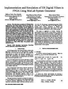
are multipliers. Maximum path delay which is highlighted is considered to be the critical path.

18 Zero delay path for filter DFG

16 14 12 10 8 6 4 2 0 1

2

3 4 Vertex number in filter DFG

5

Figure 7: Zero path delays and critical path for 4th-order low pass elliptic filter.

path matrix. These signals, in this matrix, are output as the critical path. The state 𝑆8 is provided to enable looping action and for updating all the signals. The state machine then goes back to state 𝑆0 and awaits new inputs. Next, algorithm to find the shortest path between two nodes in a graph is described. For retiming technique in high level synthesis, we need the shortest path to solve system of inequalities. It is seen that time needed to compute critical path on FPGA is reasonably less when compared to computation on general purpose processor. This also reduces the retiming computation time. The zero delay paths are computed for 4th-order elliptic filter shown in Figure 7. The highlighted path delay is from1 → 9 → 5 → 14 → 8 where nodes 1, 5, 8 are adders and 9, 14

3.2. Shortest Path Solver Algorithm and State Diagram. Let 𝐷(𝑢, V) be the maximum delay between nodes 𝑢 and V and let 𝑇(𝑢, V) be total computation time of zero delay path from 𝑢 to V. We can check the condition 𝑇(𝑢, V) − min{𝑡(𝑢), 𝑡(V)} > {𝑑𝑒𝑟𝑖V𝑒𝑑 𝑐𝑙𝑜𝑐𝑘 𝑝𝑒𝑟𝑖𝑜𝑑} then select those paths to retime so that computation time in this path can be reduced. We have to retime the edges by constructing system of linear inequalities. This can be done using Floyd-Warshall shortest path algorithm Algorithm 3. This can be used for retiming the graph further (Figure 6). Floyd-Warshall all pair shortest path algorithm is designed and implemented as a part of path solvers on FPGA [17] which reduces the computational burden of general purpose processor where actual retiming has been carried out. The speed of computation is also increased by a larger extent. The HDL program for the shortest path solver on FPGA was designed based on the state diagram shown in Figure 8. Updating of the looping variables is done in 𝑆1 and then transition from 𝑆1 to 𝑆0 occurs. The transition from 𝑆0 to 𝑆2 occurs after the incidence matrix is completely copied to the signal weight temp. In state 𝑆2, the signal weight temp is operated upon to obtain the pair wise shortest path matrix with state 𝑆3 enabling looping action. Transition from 𝑆2 to 𝑆3 takes place after each pair wise path distance is found. Updating of the looping variables is done in 𝑆3 and then transition from 𝑆3 to 𝑆2 occurs. The transition from 𝑆2 to 𝑆4 occurs after all the pair wise shortest paths are stored in the signal weight temp. In the state 𝑆4, the elements of the signal matrix weight temp are copied to the output matrix.

10

VLSI Design Weight temp updated


atr i m

ce

ou tp ut

en m

to

i atr p tem ht

W eig

ig we to

ht tem p

ied op

co pi ed

xc

All pair shortest paths found

S4

Pairwise shortest path found

S2


S3


Weight temp complete array to output matrix

S1

cid In

x

S0

S3

Figure 8: Shortest path solver state diagram.

The state 𝑆5 enables looping action for 𝑆4. Transition from 𝑆4 to 𝑆0 occurs after the output matrix is available with all the inf [1 [ [2 [ [3 [ [inf [ [inf [ [inf [ [inf [ SPM = [inf [inf [ [1 [ [2 [ [inf [ [inf [ [3 [ [4 [3

0 1 1 2 inf inf inf inf inf inf 0 1 inf inf 2 3 2



0 1 2 3 3 1 2 3 0 1 1 2 2 3 3 4 3

0 1 2 3 2 3 1 2 2 0 1 2 1 2 3 4 3

0 1 2 3 1 2 3 1 1 2 1 2 0 1 3 4 2

0 1 2 3 0 1 2 3 0 1 1 2 1 0 3 4 1

3.3. Multiplierless Digital Filters. The digital FIR filters and the transposed IIR filters will have block of multipliers in the filter structure. This is shown in Figure 9. For a target set 𝑇 = {𝑡1 , 𝑡1 , . . . , 𝑡𝑛 } in digital filter, we have to find the ready set 𝑅 = {𝑟0 , 𝑟1 , . . . , 𝑟𝑚 } that is small

pair wise shortest paths. The state machine is then initialized and awaits new inputs. 0 1 2 3 inf inf inf inf inf inf 1 2 inf inf 3 4 3





0 1 2 3 0 1 2 3 0 1 1 2 2 3 3 4 3



0 1] ] 2] ] 3] ] inf ] ] inf ] ] inf ] ] inf ] inf ] ] inf ] ] 1] ] 2] ] inf ] ] inf ] ] 3] ] 4] 3]

(10)

and 𝐴𝑜𝑝𝑒𝑟𝑎𝑡𝑖𝑜𝑛 composed of minimum number of addition, subtraction, and shift operations. After this target set is obtained, multiplierless multiple constant multiplication filters can be designed with this target set. Multiple constant multiplication (MCM) is an efficient way of implementing

VLSI Design

11

Input

Multiplier block

Input

Multiplier block

Z−1 +

Z−1 +

Z−1 · · · Z−1

+

Z−1 +

+

Z−1 · · · Z−1

+ Z−1 +

Z−1

Output +

Multiplier block

Z−1 Multiplier block

Z−1

+

(a)

Z−1 · · · Z−1

+ Z−1 +

Output

Z−1

(b)

Input

Multiplier block

Z−1

+

Z−1 · · · Z−1

+

Z−1

+

Output

(c)

Figure 9: General structure of MCM block for (a) FIR filter, (b) transposed direct form-I IIR filter, and (c) transposed direct form-II IIR filter.

several constant multiplications with the input data [18, 19]. The coefficients are implemented using shifts, adders, and subtracters. By removing the redundancy between the coefficients, the number of adders and subtracters is reduced which results in a low complexity implementation. Retiming for multiplierless MCM filters is still unexplored in the literature and authors have combined retiming for multiplierless MCM filters which shows decrease in the combinational path delay. For filter graph 𝐺, multiplierless MCM filter can be designed using target set and 𝐴𝑜𝑝𝑒𝑟𝑎𝑡𝑖𝑜𝑛𝑠, and multiplierless MCM filter graph 𝐺𝑖 is obtained. This is again retimed to increase the speed performance of 𝐺𝑖 by modifying the critical path of the filter. The graph after retiming of multiplierless MCM filter is considered as 𝐺𝑟 . In the present work, 𝐻cub algorithm is used for 𝐺𝑖 computation. The input to the 𝐻cub algorithm is target set 𝑇 and algorithm computes a ready set 𝑅 which is the output solution. The 𝑅 set computation requires multiple iterations and, in each iteration, successor set 𝑆 of 𝑅 is chosen as the next fundamental based on the heuristic. Here, 𝑆 which is set of constants of distance 1 from 𝑅 is given as 𝑆 = {𝑠 | dist (𝑅, 𝑠) = 1} = 𝐴 𝑠 (𝑅, 𝑅) .

(11)

For the target set of constants 𝑇 for the considered filter graph 𝐺, using 𝐻cub algorithm compute set 𝑅 = {𝑟1 , 𝑟2 , . . . , 𝑟𝑚 } with 𝑇 ∈ 𝑅. If the targets are found in the 𝑆, then it is optimal synthesis. Here, heuristic function 𝐻(𝑅, 𝑆, 𝑇) of an algorithm can be chosen when no more targets are found in 𝑆. This can happen when all the targets are more than one 𝐴𝑜𝑝𝑒𝑟𝑎𝑡𝑖𝑜𝑛 away. The optimal part is when (𝑇 ∩ 𝑆 ≠ 𝜙), then there is a target in the successor set and it can be synthesized. Optimal set is the one in which the entire target is synthesized in this way and the solution is optimal. In heuristic part, the computation can be done by two ways: (i) maximum benefit, (ii) cumulative benefit.

To build the heuristic, we can define the benefit function as 𝐵(𝑅, 𝑠, 𝑡): 𝐵 (𝑅, 𝑠, 𝑡) = dist (𝑅, 𝑡) − dist (𝑅 + 𝑠, 𝑡) .

(12)

A successor 𝑠 ∈ 𝑆 needs to be picked which is closest to the target set to minimize the cost. This is possible if we can compute or estimate the A-Distance. It is useful to also take into account the current estimate of the distance between 𝑅 and 𝑇. Thus, to build the heuristic, we must first define the benefit function 𝐵(𝑅, 𝑠, 𝑡) to quantify to what extent adding a successor s to the ready set 𝑅 improves the distance to a fixed, but arbitrary, target 𝑡. However, for remote targets, the estimate becomes less accurate; hence, we can have weighted benefit function given as 𝐵𝑏 (𝑅, 𝑠, 𝑡) = 10dist(𝑅+𝑠,𝑡) (dist (𝑅, 𝑡) − dist (𝑅 + 𝑠, 𝑡)) ,

(13)

where 10dist(𝑅+𝑠,𝑡) is a weight factor and decreases exponentially as 𝑡 grows. The benefit function for different targets 𝑡 can be added and joint optimization can be achieved by using cumulative benefit which is used in the present work. Hence, heuristic function for cumulative benefit is given by 𝐻cub (𝑅, 𝑆, 𝑇) = arg [max [∑ 𝐵𝑏 (𝑅, 𝑆, 𝑡)]] .

(14)

𝑡∈𝑇

Here, cumulative benefit heuristic adds up the weighted benefit considering all the targets. With this particular method, target set is calculated. With this target set, filter graph which is multiplierless MCM based can be designed. It is found that multiplierless designs reduce the combinational path delays and due to sharing of intermediate results in the MCM approach. The performance can be further improved by retiming 𝐺𝑖 to give 𝐺𝑟 . These two different optimization techniques reduce the combination delay and critical path

12

VLSI Design

1 Input

+

Vy = Vu ∗ 23 Qy = Qu ≪ 3 Ey = Eu

−

+

−

+

Z−1

+

−u

−

+

+

+

Vy = Vu ∗ 21 Qy = Qu ≪ 1 Ey = Eu

Vy = Vu ∗ 25 Qy = Qu ≪ 5 Ey = Eu

Vy = Vu ∗ 21 Qy = Qu ≪ 1 Ey = Eu

−

Vy = Vu ∗ 25 Qy = Qu ≪ 5 Ey = Eu

+

Vy = Vu ∗ 25 Qy = Qu ≪ 5 Ey = Eu

+

−u

Vy = Vu ∗ 22 Qy = Qu ≪ 2 Ey = Eu

+

+

−

+

Output

+

Z−1 +

Vy = Vu ∗ 26 Qy = Qu ≪ 6 Ey = Eu

Vy = Vu ∗ 25 Qy = Qu ≪ 5 Ey = Eu

+

+

+

Z−1

+ +

1

+

+

Z−1

+

Z−1

Z−1

+

+

+

Z−1 −1

Z

Vy = Vu ∗ 21 Qy = Qu ≪ 1 Ey = Eu

+

+

Vy = Vu ∗ 25 Qy = Qu ≪ 5 Ey = Eu

Figure 10: Multiplierless MCM based 4th-order elliptic filter.

without changing the functionality which further increases the clock speed. The 4th-order lattice filter with multiplierless MCM concept using 𝐻cub algorithm is shown in Figure 10. It is seen from the synthesis that combination delay is reduced. It is further retimed either for clock period minimization or register minimization. This requires solving a set of linear inequalities with a computation complexity of 𝑂(𝑛3 ) where 𝑛 is the number of nodes using the Floyd-Warshall algorithm, where 𝑛 is the number of nodes [8]. The clock period minimization and register minimization retiming algorithms are designed and implemented with FPGA based path solvers which reduces computation time when compared to previous methods [8, 16] to design multiplierless digital filters. The algorithm starts by building a new graph from the original DFG. The new graph can give us a set of inequalities called the critical path constraints. The original DFG also presents a set of equalities called the feasibility constraints. A constraint graph can be built from the critical path constraints and the feasibility constraints. The retiming values for each node can be derived by applying a FloydWarshall shortest path algorithm to the constraint graph. The weight for each edge in the retimed DFG can be calculated using the original weight and the retiming values of the two nodes connected by this edge. The improvement in the clock

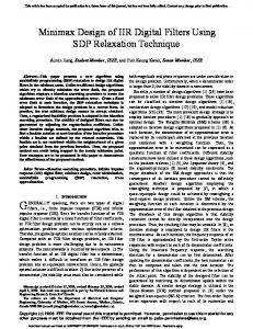
frequency is shown in Figure 11. Here, 4th-order lattice filter is considered. 𝐷𝑒𝑠𝑖𝑔𝑛1 is the filter with multipliers and without retiming, 𝐷𝑒𝑠𝑖𝑔𝑛2 is multiplierless MCM based filter without retiming, 𝐷𝑒𝑠𝑖𝑔𝑛3 is the filter with multipliers with retiming, and 𝐷𝑒𝑠𝑖𝑔𝑛4 is multiplierless MCM based lattice filter with retiming. The maximum operating frequency of the filter has increased by 19.6% in multiplierless MCM approach as multipliers will get eliminated and get replaced by adders which have much less computation delay. Further, it is observed that by combining this approach with retiming, operating frequency increases by 35.4% which is a significant increase. However, with this technique, the number of registers increases from 9 to 11. Hence, when the filter is designed without multipliers (that is using only adders/subtractors and shifters) along with the retiming technique, operating clock speed is found to increase which gives a greater speed advantage for the design under consideration. 3.4. Computer Aided Design Tool. This section presents the DiFiDOT tool which is designed as the part of research work. Initially, the design of filters is performed using retimed architecture where user can choose either clock period

VLSI Design

13 In each stage, the partial products 𝑃𝑖 are generated that are added to obtain final product 𝑃. In general, for 𝑚 ∗ 𝑛 array multiplier, we need 𝑚 ∗ 𝑛 AND gates, 𝑛 half adders, and (𝑚 − 2) ∗ 𝑛 full adders.

80 70 60 50 40 30 20 10 0 Design1

Design2

Design3

Design4

Frequency in MHz Number of registers

Figure 11: Comparison of operating frequency and number of registers for different filter designs of 4th-order elliptic filter.

minimization or register minimization retiming as per his need. The tool will retime the digital filter by optimizing the critical path and generate verilog/VHDL based filter RTL for the same. The performance of a filter can also be increased by varying the choice combinational adder and multiplier elements in the RTL filter description. A graphical user interface (GUI) is created in DiFiDOT using Nokia QT 4.8.0 for component selection and optimization of digital filters. Here, user has to input the HDL file which was automatically generated after retiming for further component optimization. The user can choose adders and multipliers of his choice according to the design requirements for the retimed digital filters using drop down menu. The original HDL is automatically modified with respect to the components chosen which is again synthesizable and is given as the output to the user. This easy to use GUI helps designer to optimize and generate digital filter RTL with the adder and multipliers of his choice. With this, designer can conveniently explore the solution space of possible architectures and also analyze the trade-offs in the energy-area-performance space [20]. The different adder and multipliers considered in the tool are as below. Multiplier Architecture. The most critical function carried out by any filter is multiplication. Digital multiplication [19] is the most extensively used operation in signal processing. Innumerable schemes have been proposed for realization of the operation. In this paper, we consider three types of multipliers. Array Multiplier. It is the basic type of multiplier. Consider two binary numbers 𝐴 and 𝐵, of 𝑛 bits, respectively. The multiplication is given as 𝑛−1

𝐴 = ∑ 𝐴𝑖 2𝑖 ,

𝑛−1

𝐵 = ∑ 𝐴𝑖 𝐵𝑖 2𝑖+𝑗

𝑖=0 𝑛 𝑛−1

𝑗=0

(15) 𝑖 𝑖 (𝑖+𝑗)

𝑃 = ∑∑𝐴 𝐵 2 𝑖=0 𝑗=0

𝑖 𝑖 𝑖+𝑗

𝐴𝐵2 .

Radix 4 Booth Multiplier. It has the advantage of lesser area and faster multiplication compared with array multiplication. Radix 4 Booths Algorithm can scan strings of three bits and is converted depending on modified Booth encoder table. The design of Booths multiplier in this project consists of four Modified Booth Encoders (MBE), four sign extension correctors, four partial product generators (comprises of 5 : 1 multiplexer), and finally a Ripple carry Adder. This Booth multiplier technique is to increase speed by reducing the number of partial products by half. Since a 32-bit booth multiplier is used in this project, there are only sixteen partial products that need to be added instead of 32 partial products generated using conventional multiplier. Vedic Multiplier. It is used for faster multiplication operations in higher order bits. It has less combinational path delay [21] compared with others when the bit size is higher. However, it consumes more area than Booth multiplier and array multiplier. The multiplier is based on an algorithm Urdhva Tiryakbhyam (vertical & crosswise) Sutra which is a general multiplication formula applicable to all cases of multiplication. It means vertically and crosswise. It is based on a novel concept through which the generation of all partial products can be done with the concurrent addition of these partial products. The speed advantage is compromised with increased power dissipation and area. Due to its regular structure, layout of this can be easily generated. The different multipliers are designed for different bit sizes and results are compared. This is as shown in Table 1.

3.5. Adders. In this paper, qualitative evaluations of the classified binary adder architectures are performed since adder is another basic component of FIR filter. Here, Ripplecarry adder, BruntKung adder, and Ling adder are considered to emphasize the performance properties. Adders affect the critical path delay and area. Ripple Adder. It is the basic adder type. This is composed of cascaded full adders for 𝑛-bit adder. It is constructed by cascading full adder blocks in series. The carry-out of one stage is fed directly to the carry-in of the next stage. For an 𝑛-bit parallel adder, it requires n full adders. Parallel-Prefix Adders. Parallel prefix adders [22] offer a highly efficient solution to the binary addition problem. Among all the parallel prefix adders, Brunt Kung adder has a good balance between area, power, and performance. It is found that Ling adder using Kogge-Stone parallel prefix adder is also having the advantage of faster addition operation [22], but it consumes more power than Brunt Kung Adder.

14

VLSI Design Table 1: Comparison of multipliers for delay, power, and area.

Type of multiplier Array Booth Vedic

32 bit 76.1 86.1 70.7

Delay in ns 16 bit 39.9 27.99 39.02

8 bit 21 14.9 24.4

32 bit 21 25 28

Power in mW 16 bit 11 15 18

8 bit 7 12 12

32 bit 1519 1277 2378

Number of LUTs 16 bit 375 317 565

8 bit 91 77 126

The basic equations used in parallel prefix adders are given below. The equations of bit generate and propagate are 𝐺0:0 = 𝐺0 = 𝑐in 𝑃0:0 = 𝑃0 = 0

(16)

𝐺𝑖:𝑗 = 𝐺𝑖:𝑘 + 𝑝𝑖:𝑘 ∗ 𝑔(𝑘−1):𝑗 𝑃𝑖:𝑗 = 𝑃𝑖:𝑘 ∗ 𝑝(𝑘−1):𝑗 . The sum generation is given by 𝑆𝑖 = 𝑃𝑖 XOR 𝐺(𝑖−1):0 .

(17)

Different Adders are designed for different bit sizes and their VLSI design metrics are compared as shown in Table 2. The delay generated is based on the combinational path delay after synthesis. It is measured in 𝑛𝑠. In the GUI, an option is crested for particular adder and multiplier combination also depending on whether the performance parameter is speed, power, or area and also based on the bit size. For example, if the design constraint that user chooses is power then Brent-Kung adder and array multiplier pair are considered as the best combination to implement the filter in the design optimization GUI. User can also choose any one of his choice among area, power, or speed constraint for digital filter HDL generation. Along with this, an option is created for multiplierless filter design description as well based on MCM approach. It is seen that the retimed MCM circuits outperform the existing MCM methods [23] in terms of speed. Using this tool, user can design retimed digital filter which has combination elements of his choice which are specific to particular design constraint and generate the RTL for the same. The obtained RTL can be synthesized with any of the commercially available synthesis tools. The GUI designed is shown in Figure 12. A 𝐻cub based algorithm is considered for implementing MCM blocks in multiplierless digital filters for specific user defined option in DiFiDOT. Since all the multipliers can be realised as a block in transposed IIR and FIR filters, they are well suited for MCM implementation. After retiming, the multiplier blocks in digital filter can be replaced by a block constructed by adderssubtractors, negation operations, and shifters in multiplierless design approach. The generated MCM block will have tree depth in terms of different components and this depth in our work is assumed to be infinity. The tool DiFiDOT automatically generates the HDL of retimed digital filter which is under consideration which can be directly synthesizable. With this tool and automation, even if reiteration of the design cycle happens due to specification change, time taken to reiterate is very little.

Figure 12: GUI for dDesign optimization environment created to generate synthesizable retimed digital filter HDL optimized for VLSI design metrics.

4. Experimental Results This section is divided in to three parts: the first part presents the results of retiming with FPGA based path solvers, second part presents comparison of various retiming techniques, and third part presents the timing results of retimed filter structures with MCM blocks. 4.1. Results on Path Solvers for Retiming. The main idea of implementing path solver algorithms on FPGA is to speed up the results for retiming purposes. The inputs are passed to the FPGA based path solver block by a processor where retiming algorithm is implemented. The computations are performed in FPGA based block and shortest path along with critical path is computed and communicated back to the processor where retiming will be performed. For comparison, a set of designs is used to test the path solver algorithms. The designs are a diverse set of DSP functions of varying complexity which includes recursive and nonrecursive filter structures. The considered target device for path solver implementation is Spartan6 family based XC6SSLX16. The simulation and synthesis of path solvers are performed using Xilinx ISE tool suit and the synthesis and the timing results after synthesis are shown in Table 1. The FPGA based path solver computes critical path and shortest path and communicates the results to the processor where retiming is performed. This reduces the burden on main processor (Table 3).

VLSI Design

15 Table 2: Comparison of adders for delay, power, and area.

Type of adder Ling BrentKung Ripple

32 bit 8.854 10.4 12.12

Delay in ns 16 bit 15.24 18.39 20.63

8 bit 20.21 25.83 37.6

32 bit 6 4 2

Power in mW 16 bit 9 6 7

8 bit 18 9 14

32 bit 23 15 9

Number of LUTs 16 bit 53 30 18

8 bit 107 63 36

Table 3: Device utilization and timing summary of path solvers.

Min period in ns

Timing summery Setup time in ns

Hold time in ns

9.068 ns

15.72 ns

6.141 ns

110.277

14.089 ns

10.477 ns

4.114 ns

70.978

4.2. Comparison of Clock Period Minimization and Register Minimization Retiming Technique. Different filter structures are designed and they are compared with respect to the clock period and register count before and after retiming. It is observed that after retiming, the clock period gets reduced. The register count gets altered depending on the filters iteration bound. Here, three models are considered. 𝑀𝑜𝑑𝑒𝑙1 is the filter without retiming and with adder, subtractor, multiplier, and delay elements. 𝑀𝑜𝑑𝑒𝑙2 is retimed filter based on clock period minimization algorithm. 𝑀𝑜𝑑𝑒𝑙3 is retimed filter based on register minimization algorithm. After retiming, the results are compared with the original circuit [24]. The comparison results are shown in Figure 13. After retiming, the finite state machine is extracted from the retimed circuit and it is compared with original circuit for its functionality. It is observed that clock period minimization retiming algorithm is efficient in terms of reduction critical path, thereby increase in the clock frequency. However, this

Max. frequency (Hz)

40 35 30 25 20 15 10 5

Model 1 clock period Model 1 reg count Model 2 clock period

FIR-12

IIR-12

FIR-10

IIR-10

FIR-8

IIR-8

FIR-6

IIR-6

FIR-4

IIR-4

0 FIR-2

Here, various IIR and FIR filters have been considered to analyze the FPGA based path solvers and execution time of FPGA design is compared with the general purpose processor (GPP) based design. Also, GPP denotes the required CPU time in milliseconds of the path solver to find the minimum solution on a PC with Intel Pentium 5 machine at 2 GHz and 4 GB of memory. FPGA based design solves for critical path and shortest path in very less time when compared to the general purpose processor based path solvers. The time taken by the FPGA path solvers is compared in Table 4 to the time taken by the algorithms run using general purpose processor with Matlab environment. The time overhead needed for general purpose processor where retiming algorithm is implemented in MATLAB to communicate with the FPGA based path solvers is around 210 ns for each computation. Including this, the time gain achieved is quite substantial when compared to designs without FPGA based path solvers. These time gains are good and can really help speed up the results, which is crucial for retiming.

IIR-2

Device utilization summery Logic utilization Used Number of slices 5804 Critical path solver Number of LUTs 10462 Number of slice Flipops 3664 Number of slices 4147 Shortest path solver Number of LUTs 7511 Number of slice Flipops 1496 Path solver name

Model 2 reg count Model 3 clock period Model 3 reg count

Figure 13: Clock period and register count before and after retiming for various digital filter blocks.

might increase the register count. In register minimization retiming [18], the number of registers after retiming will be reduced while compromising the clock period. 4.3. Area, Power, and Timing Results for Digital Filter before and after Retiming for Different Adder and Multiplier Combinations. The FIR and IIR filters are designed with respect to different adders and multipliers combinations. As an application example, IIR and FIR filters [25] of order 10 are considered. Table 5 shows the results of FIR/IIR filters before and after retiming for particular adder and multiplier combinations. User can choose any adder and multiplier for the filter circuit depending on the design requirement. In

16

VLSI Design Table 4: Computation time comparison.

Filter order

2 4 6 8 10 12

Critical path solver algorithm IIR filter FIR filter FPGA based GPP based FPGA based GPP based (ns) (ms) (ns) (ms) 4.60 13.8 9.06 12.83 15.71 15.78 16.31 14.46 29.98 19.18 19.23 15.47 31.62 21.90 29.71 16.42 39.81 26.27 36.53 18.61 46.72 31.42 43.28 23.52

Shortest path solver algorithm IIR filter FIR filter FPGA based GPP based FPGA based GPP based (ns) (ms) (ns) (ms) 2.78 3.05 3.05 12.80 3.68 13.91 13.91 13.19 3.98 15.42 15.42 17.31 4.52 25.23 25.23 32.94 5.36 42.93 42.93 45.34 6.71 55.34 55.34 51.61

Table 5: Comparison results of different adder/multiplier combinations for digital filters.

Number of LUTs

After retiming Max. operating freq in MHz

Power in mw

Brentkung Adder/Array Multiplier Ling Adder/Vedic Multiplier Ripple carry Adder/Booth Multiplier

2222 2214

62.526 69.702

99 112

2411 2193

76.977 95.381

89 94

2146

50.861

114

1809

65.248

95

Brentkung Adder/Array Multiplier Ling Adder/Vedic Multiplier Ripple carry Adder/Booth Multiplier

1736 2162

62.526 72.493

94 111

1811 2271

99.43 100.72

85 95

1637

52.302

105

1615

71.345

87

All the three models are compared for the performance parameters such as area, power, and delay. Here, it is ensured that functionality of the circuits after and before retiming is retained. The frequency improvement seen for different filters by considering the above models is given in Figure 14. It is seen that frequency parameter is improved when retiming technique is applied for multiplierless MCM based digital filters.

70 60 50 40 30 20

IIR-12

IIR-10

IIR-8

IIR-6

IIR-4

IIR-2

0

FIR-12

10 FIR-10

(i) 𝑀𝑜𝑑𝑒𝑙 1: Filter with adder, multiplier, and delay elements. (ii) 𝑀𝑜𝑑𝑒𝑙 2: Filter based on multiplierless multiple constant multiplication approach. (iii) 𝑀𝑜𝑑𝑒𝑙 3: Retimed multiplierless multiple constant multiplication based filter.

80

FIR-8

4.4. Results for Optimization of Latency, Multiplier Components, and Power in Multiplierless Multiple Constant Multiplication Based Filter Designs Using Retiming Algorithm. Table 6 presents the results of the filters designed using multiplierless MCM approach and optimization using retiming algorithm. Here, 3 models are used.

90

FIR-6

the GUI, particular adder and multiplier combination is considered depending on whether the performance parameter is delay, power, or area and also based on the bit size. If user does not want to use these in built combinations, user can choose any one of his choice among the available for FIR/IIR digital filter HDL generation with specific combinational components.

FIR-4

FIR-10

Before retiming Number Max. operating Power in of LUTs freq in MHz mw

FIR-2

IIR-10

Adder/multiplier combinations

Frequency improvement (%)

Filter block

Filter type Frequency improvement from model 1 to model 2 Frequency improvement from model 1 to model 3

Figure 14: Frequency improvement in % factor.

5. Application Example The electrocardiogram (ECG) is the most commonly used diagnostic method for heart diseases. Good quality ECG is utilized by physicians for interpretation and identification of physiological and pathological phenomena. ECG recordings

VLSI Design

17 Table 6: Comparison of area, delay, and power for different models of various digital filters. Adder multipliers Flipflops Model 1 Model 2 Model 3 5/2/3 5/0/3 5/0/4 10/3/5 11/0/5 11/0/8 7/2/7 17/0/7 17/0/14 15/5/9 22/0/9 22/0/16 18/6/11 25/0/11 25/0/11 20/7/13 29/0/13 29/0/13 9/4/3 11/0/3 11/0/3 16/7/5 20/0/5 19/0/6 24/11/7 35/0/7 35/0/8 30/11/10 33/0/10 33/0/7 37/16/13 54/0/13 54/0/14 42/20/17 63/0/17 63/0/19

Filter block FIR-2 FIR-4 FIR-6 FIR-8 FIR-10 FIR-12 IIR-2 IIR-4 IIR-6 IIR-8 IIR-10 IIR-12

DelayMax Freq in MHz Model 1 Model 2 Model 3 51.54 192.14 340.62 59.41 108.41 222.04 62.91 67.64 259.47 54.82 65.92 117.91 48.22 56.37 100.72 46.34 54.86 193.40 55.03 75.53 89.10 22.78 113.88 151.65 38.71 42.54 53.142 29.46 70.14 110.21 36.43 48.85 95.381 39.73 50.74 101.52

Model 1 0.056 0.047 0.051 0.054 0.058 0.060 0.047 0.059 0.051 0.044 0.051 0.063

Power in Watts Model 2 Model 3 0.063 0.065 0.057 0.060 0.062 0.064 0.058 0.065 0.061 0.063 0.063 0.067 0.050 0.050 0.062 0.063 0.059 0.058 0.064 0.081 0.067 0.085 0.071 0.088

DSP

Noise 1 + + Add 1

In 1

Out 8 Scope 3

DSP

Filter 2

ECG 1 (a)

(b)

Figure 15: Structure of ECG block for power noise removal; (a) block diagram; (b) filter block expanded.

are often corrupted by high-frequency noises, such as powerline interference, electromyography (EMG) noise, and instrumentation noise. An ECG is usually affected by the 50/60 Hz noise in the power supply lines. This noise can be eliminated by using a digital filter. The model is constructed in matlab and tested for ECG signals for removing the noise. The constructed model uses retimed multiplierless MCM filter which is implemented on FPGA and tested for ECG signal which is corrupted by power-line noise. The filter efficiently filters out the noise and outputs the clean ECG signal. The ECG noise removal block using the optimized filter structure is shown in Figure 15.

6. Conclusions In this paper, we introduced the retiming approach for designing multiplierless MCM based digital filters with speed and area as the constraint. The implementation cost at the gate level is reduced by using addition, subtraction, and shift operations instead of multiplication and by using register sharing and register minimization retiming algorithm approach. Since there are still instances with which multiplierless designs can not cope, we also proposed

the combination of adder and multiplier blocks which can be used in retimed filter design which is applicable for specific VLSI design constraint such as power, area, and timing. This yields the optimal clock speed and gate-level area in design and implementation of digital filters. This paper also introduced the design architectures for the digital filter and a CAD tool for the realization of retimed digital filters which can be either multiplierless MCM based or with adder/subtractor, multiplier, and delay elements. This tool directly gives the synthesizable filter RTL which reduces lot of designers’ time and effort in the design cycle. The experimental results indicate that the retiming algorithm efficiency can be further increased by using FPGA based path solver algorithms proposed in this paper. It was shown that the realization of path solver architectures for solving critical path and shortest path in retiming computation and communicating the results to the processor where retiming algorithm is implemented yields significant increase in computation time gain when compared to the filter designs for which path solver algorithms are implemented as a part of retiming algorithm in the processor. It is observed that a designer can find the synthesizable digital filter RTL that fits best in an application.

18

Conflict of Interests The authors declare that there is no conflict of interests regarding the publication of this paper.

References [1] C. Soviani, O. Tardieu, and S. A. Edwards, “Optimizing sequential cycles through shannon decomposition and retiming,” IEEE Transactions on Computer-Aided Design of Integrated Circuits and Systems, vol. 26, no. 3, pp. 456–467, 2007. [2] S. Bommu, N. O’Neill, and M. Ciesielski, “Retiming-based factorization for sequential logic optimization,” ACM Transactions on Design Automation of Electronic Systems, vol. 5, no. 3, pp. 373–398, 2000. [3] K. K. Parhi, “A systematic approach for design of digit-serial signal processing architectures,” IEEE Transactions on Circuits and Systems, vol. 38, no. 4, pp. 358–375, 1991. [4] D. Yagain, A. V. Krishna, and S. Chennapnoor, “Design optimization platform for synthesizable high speed digital filters using retiming technique,” in Proceedings of the 10th IEEE International Conference on Semiconductor Electronics (ICSE '12), pp. 551–555, Kuala Lumpur, Malaysia, September 2012. [5] N. Shenoy, “Retiming: theory and practice,” Integration, the VLSI Journal, vol. 22, no. 1-2, pp. 1–21, 1997. [6] C. E. Leiserson and J. B. Saxe, “Retiming synchronous circuitry,” Algorithmica, vol. 6, no. 1–6, pp. 5–35, 1991. [7] Y. Tsao and K. Choi, “Area-efficient VLSI implementation for parallel linear-phase FIR digital filters of odd length based on fast FIR algorithm,” IEEE Transactions on Circuits and Systems II: Express Briefs, vol. 59, no. 6, pp. 371–375, 2012. [8] K. K. Parhi, VLSI Digital Signal Processing Systems: Design and Implementation, John Wiley & Sons, 2007. [9] K. K. Parhi, “Hierarchical folding and synthesis of iterative data flow graphs,” IEEE Transactions on Circuits and Systems II: Express Briefs, vol. 60, no. 9, pp. 597–601, 2013. [10] X. Zhu, T. Basten, M. Geilen, and S. Stuijk, “Efficient retiming of multirate DSP algorithms,” IEEE Transactions on ComputerAided Design of Integrated Circuits and Systems, vol. 31, no. 6, pp. 831–844, 2012. [11] N. Liveris, C. Lin, J. Wang, H. Zhou, and P. Banerjee, “Retiming for synchronous data flow graphs,” in Proceedings of the Asia and South Pacific Design Automation Conference (ASP-DAC '07), vol. 7, pp. 480–485, Yokohama, Japan, January 2007. [12] N. L. Passos, E. H. Sha, and S. C. Bass, “Optimizing DSP flow graphs via schedule-based multidimensional retiming,” IEEE Transactions on Signal Processing, vol. 44, no. 1, pp. 150–155, 1996. [13] J. R. Jiang and R. K. Brayton, “Retiming and resynthesis: a complexity perspective,” IEEE Transactions on Computer-Aided Design of Integrated Circuits and Systems, vol. 25, no. 12, pp. 2674–2686, 2006. [14] N. Maheshwari and S. Sapatnekar, “Efficient retiming of large circuits,” IEEE Transactions on Very Large Scale Integration (VLSI) Systems, vol. 6, no. 1, pp. 74–83, 1998. [15] D. Yagain and A. Vijaya Krishna, “High speed digital filter design using register minimization retiming & parallel prefix adders,” in Proceedings of the 3rd International Conference on Emerging Applications of Information Technology (EAIT ’12), pp. 449–453, Kolkata, India, December 2012.

VLSI Design [16] J. Cong and C. Wu, “An efficient algorithm for performanceoptimal FPGA technology mapping with retiming,” IEEE Transactions on Computer-Aided Design of Integrated Circuits and Systems, vol. 17, no. 9, pp. 738–748, 1998. [17] D. Yagain, A. Vijayakrishna, P. Nikhil, A. Adarsh, and S. Karthikeyan, “FPGA based path solvers for DFGs in high level synthesis,” in Proceedings of the 2nd International Conference on Advances in Computational Tools for Engineering Applications (ACTEA ’12), pp. 273–278, IEEE, Beirut, Lebanon, December 2012. [18] Y. Voronenko and M. P¨uschel, “Multiplierless multiple constant multiplication,” ACM Transactions on Algorithms, vol. 3, no. 2, article 11, Article ID 1240234, 2007. [19] K. Johansson, O. Gustafsson, and L. Wanhammar, “Multiple constant multiplication for digit-serial implementation of low power FIR filters,” WSEAS Transactions on Circuits and Systems, vol. 5, no. 7, pp. 1001–1008, 2006. [20] A. Baliga, “Design of high-speed adders for efficient digital design blocks,” ISRN Electronics, vol. 2012, Article ID 253742, 9 pages, 2012. [21] H. D. Tiwari, G. Gankhuyag, C. M. Kim, and Y. B. Cho, “Multiplier design based on ancient indian vedic mathematics,” in Proceedings of the International SoC Design Conference (ISOCC ’08), vol. 2, pp. II65–II68, Busan, Republic of Korea, November 2008. [22] G. Dimitrakopoulos and D. Nikolos, “High-speed parallelprefix VLSI ling adders,” IEEE Transactions on Computers, vol. 54, no. 2, pp. 225–231, 2005. [23] L. Aksoy, E. da Costa, P. Flores, and J. Monteiro, “Exact and approximate algorithms for the optimization of area and delay in multiple constant multiplications,” IEEE Transactions on Computer-Aided Design of Integrated Circuits and Systems, vol. 27, no. 6, pp. 1013–1026, 2008. [24] M. N. Mneimneh, K. A. Sakallah, and J. Moondanos, “Preserving synchronizing sequences of sequential circuits after retiming,” in Proceedings of the Asia and South Pacifi c Design Automation Conference, pp. 579–584, IEEE Press, 2004. [25] D. Yagain and K. A. Vijaya, “Fir filter design based on retiming and automation using vlsi design metrics,” in Proceedings of the International Conference on Technology, Informatics, Management, Engineering, and Environment (TIME-E ’13), pp. 17–22, IEEE, 2013.

International Journal of

Rotating Machinery

Engineering Journal of

Hindawi Publishing Corporation http://www.hindawi.com

Volume 2014

The Scientific World Journal Hindawi Publishing Corporation http://www.hindawi.com

Volume 2014


Distributed Sensor Networks

Journal of

Sensors Hindawi Publishing Corporation http://www.hindawi.com

Volume 2014


Volume 2014


Volume 2014

Journal of

Control Science and Engineering

Advances in

Civil Engineering Hindawi Publishing Corporation http://www.hindawi.com


Volume 2014

Volume 2014

Submit your manuscripts at http://www.hindawi.com Journal of

Journal of

Electrical and Computer Engineering

Robotics Hindawi Publishing Corporation http://www.hindawi.com


Volume 2014

Volume 2014

VLSI Design Advances in OptoElectronics


Navigation and Observation Hindawi Publishing Corporation http://www.hindawi.com

Volume 2014



Chemical Engineering Hindawi Publishing Corporation http://www.hindawi.com

Volume 2014

Volume 2014

Active and Passive Electronic Components

Antennas and Propagation Hindawi Publishing Corporation http://www.hindawi.com

Aerospace Engineering


Volume 2014


Volume 2014

Volume 2014




Modelling & Simulation in Engineering

Volume 2014


Volume 2014

Shock and Vibration Hindawi Publishing Corporation http://www.hindawi.com

Volume 2014

Advances in

Acoustics and Vibration Hindawi Publishing Corporation http://www.hindawi.com

Volume 2014