Abstract: 3D reconstruction applications can benefit greatly from knowledge about coplanar feature points. Extracting this knowledge from images alone is a ...
DETECTING COPLANAR FEATURE POINTS IN HANDHELD IMAGE SEQUENCES Olaf K¨ahler and Joachim Denzler Department of Mathematics and Computer Science, Friedrich-Schiller-University, Jena, Germany {kaehler,denzler}@informatik.uni-jena.de
Keywords:
Planar patches, homography, degenerate motion.
Abstract:
3D reconstruction applications can benefit greatly from knowledge about coplanar feature points. Extracting this knowledge from images alone is a difficult task, however. The typical approach to this problem is to search for homographies in a set of point correspondences using the RANSAC algorithm. In this work we focus on two open issues with a blind random search. First, we enforce the detected planes to represent physically present scene planes. Second, we propose methods to identify cases, in which a homography does not imply coplanarity of feature points. Experiments are performed to show applicability of the presented plane detection algorithms to handheld image sequences.
1
INTRODUCTION
Planar structures are abundant in man-made environments and impose strong geometric constraints for the points on them. They have caught the interest of research before, and a typical application is the representation of video data as independent layers (Baker et al., 1998; Odone et al., 2002) or the interpretation of 3D scene structure (Gorges et al., 2004). Also, for geometric reconstruction tasks, planar structures play an important role. E.g. incorporation of the coplanarity constraints into a point based reconstruction algorithm has been explored (Bartoli and Sturm, 2003) and computing 3D planes from 2D homographies is possible (Rother, 2003). To benefit from coplanarity in 3D reconstruction, it is necessary to detect the planar structures from 2D information alone. A central concept for the identification of coplanar features in image sequences is the plane induced homography (Baker et al., 1998). Planar regions are mapped from one image of the sequence to another by a 2D-2D projective mapping, also called collineation or homography. This key idea has been used before to search for dominant homographies in a set of point correspondences using random sampling consensus and related techniques (Odone et al., 2002; Lourakis et al., 2002; Gorges et al., 2004; K¨ahler and Denzler, 2006). While the mentioned works purely rely on a sparse set of correspondences, other, computationally more intensive methods concentrate on an accurate
segmentation and delineation of the planes using region growing algorithms and dense matching (Fraundorfer et al., 2006). Our work is settled among the fast, actually real-time algorithms using only sparse correspondences. The addressed problems, however, are inherent to the usage of homographies in general, independent of the method actually used. While a homography might cover coplanarity in a geometrical sense, the actually interesting, physically present scene planes are only a small subset of all possibly coplanar point sets. A blind search as in RANSAC will therefore detect spurious, “virtual” planes, which was also recognized in previous research (Gorges et al., 2004). We present a more rigorous analysis of the problem in section 3, leading to a theoretically justified side condition in plane search. Although the homography is a necessary criterion for planar regions, it is not a sufficient one (K¨ahler and Denzler, 2006). To give a very simple example, all points are mapped by a common homography, the identity, between two images of a static camera. Yet not all the points need to be on one plane. Coplanarity of points can only be detected, if the optical center has moved between two images. As cases with a static or a purely rotating camera are abundant in handheld image sequences, zero camera translations have to be identified automatically and a detection of false planes has to be prevented then. In section 4, we outline the analysis of (K¨ahler and Denzler, 2006) and extend it by model selection criteria (Torr et al.,
447
VISAPP 2007 - International Conference on Computer Vision Theory and Applications
1999). An experimental performance evaluation and comparison of the approaches is provided in section 5.
2
DETECTING PLANES
To detect planar regions in an image sequence, at first point correspondences are established between two images of the sequence. In this work, we use KLT-tracking (Shi and Tomasi, 1994), which seems appropriate for e.g. 30 frames/sec and typical motion speeds of handheld cameras. For plane detection, we analyze the motion of the points between two, not necessarily successive frames. The key idea for detection of coplanarity then is to find homographies. It is well known that planar scene areas observed in two different views with a perspective camera are related to each other by a homography. Hence we can define the task of detecting a planar patch as finding “a set of points that is transferred between two images by a common homography”.
2.1 Basic Ransac In the task of finding planes, it is intuitive to take care of points off the plane. If finding the plane induced homography is considered an estimation problem, the points off the plane are outliers and methods of robust estimation can be applied. In particular the RANSAC approach seems to be the method of choice for this problem, and it was also used in previous works (Gorges et al., 2004; Lourakis et al., 2002). The RANSAC approach generates hypotheses by selecting a minimum number of random points, such that a homography can be estimated. These are typically four points with no three of them being collinear. Approaches with three points are possible, but require additional constraints like known epipolar geometry (Lourakis et al., 2002) and are not used here. Once the homography induced by the hypothesis is computed, the point correspondences supporting this hypothesis can be counted. The supporting points are those correctly transferred by the homography up to e.g. 2 pixels accuracy. Many hypotheses are generated and in the end the homography supported by the largest number of point correspondences is kept. This is called the dominant homography or plane (Odone et al., 2002; Gorges et al., 2004).
tion of the set of points into planes. Once a dominant homography is found, the points supporting it are removed and another dominant homography is computed for the remaining points. This is iterated until no more homographies can be established.
3
PLANES TO AVOID
Up to now, a blind search is employed to detect all kinds of coplanar points. This can not be enough to identify physically present scene planes, as is shown in figure 1. “Virtual” planes are detected there. These do actually consist of coplanar points, but the geometric plane containing the points does not correspond to any physical plane in the scene. With the purely geometric definition of coplanarity used so far, it is not possible to distinguish “virtual” planes from physical scene planes. On first sight, the points on virtual planes seem to be distributed along two lines, as in figure 1. But as the virtual plane intersects a third or fourth physical scene plane, a third or fourth line distribution will result. On a closer look, the physical planes we are interested in are contiguous 2D entities in 3D space, and as such they are mapped to contiguous 2D areas in the observed images. The definition of a planar patch is hence extended to “a set of points in a closed region that is transferred between two images by a common homography”. This enforces validity of the homography for the whole closed region, and not only at some of its outlines. Various strategies can be used to implement this definition algorithmically. Constructing a dense set of matches while using region growing might be one solution (Fraundorfer et al., 2006). The closed region constraint is then directly enforced by the region growing algorithm. Working only on a sparse set of correspondences, the problem was approached by picking the four seed points of RANSAC in a local neighborhood (Gorges et al., 2004). Thus it is likely to compute the homography of a physical plane, and
2.2 Iterative Dominant Homography It is straight forward to extend this in order to get a decomposition of all the observed point correspondences into several homographies, or a decomposi-
448
Figure 1: Detection of a “virtual” plane, that contains coplanar points but does not correspond to any physical plane.
DETECTING COPLANAR FEATURE POINTS IN HANDHELD IMAGE SEQUENCES
that all other points conforming the homography are on the same physical plane. The idea used in this work is to pick all point correspondences in a closed area of the image as seed points. This is achieved by starting from one random point and then iteratively adding the closest known point correspondences, until a homography can be computed. Approaching a dense set of correspondences, it is more and more certain that the detected planes correspond to physical scene planes.
4
NO CAMERA TRANSLATION
The use of homographies introduces another problem to plane detection. Homographies are a necessary criterion for coplanarity, but not a sufficient one. In case of a camera rotation or zoom without a translation of the optical center, no information on coplanarity can be inferred. This can also be derived from the following standard decomposition of a homography H: 1 (1) H = αK2 (R + tnT )K−1 1 d where K1 and K2 are the intrinsic camera matrices, R and t are the relative motion and n and d are the plane normal its distance from the origin. If and only if t = 0, a difference in plane normals n does not influence the homography H. We hence extend the definition of a planar patch to “a set of points in a closed region that is transferred by a common homography in case of non-zero camera translation”. Several methods were proposed to identify a non-zero camera translation (Torr et al., 1999; K¨ahler and Denzler, 2006). A short overview of the different approaches is given in the following, in order to show applicability to our problem and motivate the experimental comparison performed in section 5.
4.1 Homography Decomposition A first idea is to analyze a single homography matrix and check for both the terms of the decomposition (1). The term tnT is not present if there was no camera translation t = 0 or if the homography was induced by the plane at infinity n = 0. Although these two cases can not be disambiguated, using only knowledge of a single homography allows to handle independently moving scene planes, which will not be the case for the methods presented later on. In the simplest case, the intrinsic camera matrices K1 and K2 are known. The matrix H′ then expresses the homography in camera coordinates: 1 T H′ = K−1 2 HK1 = α(R + tn ) d
If and only if t = 0 or n = 0, H′ is a scaled rotation matrix αR, and all singular values of H′ are equal. Testing for a translational part in H can hence be achieved by computing the ratio of largest to smallest singular value of H′ , which will be 1 for t = 0. Frequently the intrinsic camera parameters are unknown, but known to be constant. In such cases a slightly different analysis of H can be used. The matrices H and H′ will be related by a similarity relation, i.e. they will have the same determinant, eigenvalues and some more properties, which can be found in any linear algebra textbook. Again if t = 0 then H′ is a scaled rotation matrix, all eigenvalues of H will have the same absolute value, and the ratio of largest to smallest absolute eigenvalue will be 1. This is not a two way implication, as was pointed out in (Torr et al., 1999). In the case of nT RT t = 0, the triple absolute eigenvalue of 1 will follow for arbitrary t. For both criteria, small deviations from the ratio of 1 can be allowed to cope with noisy correspondences and inaccurate homographies. An experimental evaluation of the detection rate vs. false alarms with different thresholds is given in section 5.2.
4.2 Global Homography If no knowledge about the intrinsic parameters is available, analyzing on-plane information for a single homography matrix can not be sufficient for deciding, whether a camera translation was present or not. E.g. with a QR-decomposition, any homography matrix H can be decomposed into a rotation R and an upper triangular matrix K2 . The term tnT from equation (1) is not necessary. Using off-plane information however, a static scene has to be assumed. An intuitive idea is to check, whether all observed points conform with the same homography (Fraundorfer et al., 2006). In cases with just one scene plane visible, such a test will fail. The only other cases with a global homography are a pure rotation and change of intrinsics without translation. Hence, if the dominant homography from section 2.2 is valid for almost all points, we can assume that no camera translation was present. A small amount of outliers should be tolerated, however, to handle incorrect point correspondences. As before, this introduces an adjustable threshold and a trade-off between detection and false alarm rates. An experimental evaluation is given in section 5.2.
4.3 Model Selection Detecting degenerate camera motions without adjusting thresholds would be an appealing alternative. We
449
VISAPP 2007 - International Conference on Computer Vision Theory and Applications
will therefore investigate statistical model selection approaches in this context (Torr et al., 1999; Kanatani, 2004). The basic idea is to select, whether the global homography or the epipolar geometry model is better suited to explain the observed point correspondences. In a sense, this is the global homography criterion of above with the threshold determined automatically, depending on the performance of epipolar geometry. Hence these methods can also be used in case of unknown intrinsic parameters and they will also fail in case of only one plane visible. To apply model selection, first the two models are instantiated with the respective optimal parameters. The most dominant homography is used as before and the epipolar geometry is established using RANSAC and the normalized 8-Point-Algorithm. The residuals (M) εi for point i ∈ [1 . . . N] using model M can then be computed. It is not sufficient to compare these residuals, as models with more degrees of freedom will usually adapt better to the observed data. The costs for using model M have to be considered, and the task is to select Mˆ explaining the correspondences with least residuals and least number of parameters k(M) . To handle constraints of different dimensionality, geometric model selection criteria have been developed (Kanatani, 2004; Torr, 1997). As a key, the i-th point correspondence has to be considered as a vector (xi , yi , x′i , y′i ) with D = 4 degrees of freedom. The homography model constraints a point (xi , yi ) onto a corresponding point (x′i , y′i ), and hence is a model of dimension d (H) = 2. The epipolar geometry in contrast restricts a point only onto a corresponding epipolar line, and as a third parameter is needed to define the whole correspondence, this is a model of dimension d (F) = 3. The residuals can only be measured in the dimensions actually constrained by the model. To compensate for these different residual measurements, the degrees of freedom in the correspondences d (M) have to influence the overall costs as well. Further the noise disturbing the point correspondences has to be known in order to establish a relation (M) between the residuals εi , the number of parameters k(M) and the dimensionality d (M) of a model. If an isotropic normal distribution is assumed, the standard deviation σ can be estimated as the expected residual of the most general model F (Kanatani, 2004): N
σ2 =
(M∗ )2
∑ εi
i=1
D − d (M
∗)
�
N − k(M
∗)
Now the cost of a model is a weighted sum of all the mentioned contributions, and the model with least cost is selected. Different weightings have been pro-
450
Table 1: Various values for γ1 and γ2 found in model selection literature.
Name GAIC (Kanatani, 2004) GBIC1 (Torr, 1997) GBIC2 (Torr et al., 1999) GMDL (Kanatani, 2004)
γ1 2 2 ln 4 2 − ln σS2
γ2 2 2 ln N ln(4N) 2 − ln σS2
posed, however. They can be summarized as: (M)2
εi + γ1 d (M) N + γ2 k(M) 2 i=1 σ N
Cost(M) = ∑
(2)
with γ1 and γ2 from table 1. In the GMDL criterion, the image size S is explicitly used to avoid influences from different scalings. These methods are easily applied to our problem of identifying camera translation. If the homography is a “cheaper” model than the epipolar geometry, in the sense of fitting the observed correspondences comparably accurate but with fewer degrees of freedom, we assume a zero camera translation was responsible for that global homography. In section 5.2, the performance of different γ1 and γ2 will be compared to each other and to the thresholded criteria.
5
EXPERIMENTS
Our proposed methods directly tackle the mentioned problems of plane detection, and hence allow the detection of coplanarity in a much wider range of scenarios. To demonstrate the overall performance in practical applications, we present an experimental evaluation of the algorithms. First, the basic setup of the experiments and qualitative results are shown, then in section 5.2 the methods for detection of camera translation are compared.
5.1 Qualitative Evaluation For the evaluation, two types of scene setups were used. The first of them can be considered rather artificial, showing an office environment with checkerboard patterns placed in the scene. These patterns are used only to provide good features for the point tracker, they are not needed in the further processing steps. The second set is made up from architectural scenes of model buildings. Examples from the sequences with detected planes are shown in figures 2 and 3. Note that for visualization, a convex hull of the coplanar points was computed. Not all the pixels within these polygons satisfy the coplanarity constraints, as can be seen e.g.
DETECTING COPLANAR FEATURE POINTS IN HANDHELD IMAGE SEQUENCES
Figure 2: Excerpts of a calibration pattern scene with planar patches detected in the individual frames shown as polygons with thick boundary lines.
Figure 3: Excerpts of an architectural scene with the polygons delineating planar patches found from point correspondences.
at the chimneys on top of the roof in figure 3. Also, finding the exact delineations of the planes is beyond the scope of this work. Provided only information at the sparse feature points however, the results are fairly accurate, and especially the detected planes correspond to physical scene planes.
5.2 Detecting Cases Without Translation While for the plane detection itself, a ground-truth based analysis is hardly possible, the detection of camera translation can be evaluated accurately. Using a motorized zoom and a tripod, image sequences were recorded with purely rotating, zooming and generally moving camera. These motion classes were labeled by hand, allowing a comparison of the algorithms’ performance with ground truth data. The sample graph in figure 4 shows the confidence of various criteria in a translational motion over the frames of an image sequence. Note the cases with static camera are clearly identified by all criteria. Also the higher peaks in the frames with general motion allow to identify the camera translation. Several of the criteria need a threshold for deciding the type of camera motion. As usual, this leads to a tradeoff between sensitivity and specificity, which is illustrated in a ROC-curve in figure 5. Also the
detection vs. false alarm rate of the model selection criteria is shown for comparison. In this evaluation, the frames with zooming cameras were ignored, as they can not be handled by the singular and eigenvalue criteria. The other methods work equally well for identification of purely zooming cameras. The global homography criterion seems to outperform the others for a wide range of thresholds. If no static scene can be assumed and one of the homography decomposition approaches is used, the eigenvalue criterion seems to be the best choice. The model selection criteria GAIC and GBIC1, differing only slightly in the choice of γ2 , show almost exactly the same performance. Reasonable thresholds were marked for the criteria requiring one. For the global homography criterion, 12% of outliers are tolerated, for the homography decomposition based criteria, a ratio of largest to smallest singular or eigenvalue of less than 1.17 was a good indicator for a pure rotation matrix.
6
CONCLUSIONS
Searching for homographies in point correspondences is a simple, but effective method of detecting coplanar feature points. As a novelty, we presented an analysis of situations, where the blind search or even where a
451
VISAPP 2007 - International Conference on Computer Vision Theory and Applications
correspondences. 24(4):395–406.
singular eigenenval global GMDL
Image and Vision Computing,
confidence in translation
Gorges, N., Hanheide, M., Christmas, W., Bauckhage, C., Sagerer, G., and Kittler, J. (2004). Mosaics from arbitrary stereo video sequences. In Proc. 26th DAGM Symposium, pages 342–349, Heidelberg, Germany. Springer-Verlag.
0
50
100
150
200
frame
Figure 4: Confidence of different criteria in a camera translation. White background indicates static camera, yellow background a pure rotation and green background a general motion including translation.
homography does not suffice to identify planes. First we enforced that the purely geometric homographies represent physical scene planes, then the case of a global homography resulting from zero camera translation was analyzed. Finally, the overall effectiveness of plane detection was shown in experiments. Defining coplanarity only via the geometric transfer function of a homography, it is not possible to decide, whether a plane is only geometrically present or corresponding to a physical scene plane. The key idea was to use points in a closed image area for the definition of planar patches, as the contiguous 3D plane surfaces have to be mapped to contiguous 2D areas. Finally, planes can not be detected in every situation. If there was no camera translation between two frames and the optical centers are identical, no information on coplanarity can be gained. Demanding validity of the detected homographies for frames with non-zero camera translation allows to handle this degeneracy. An automatic classification of the camera motion allows the detection of coplanar feature points also in handheld image sequences.
K¨ahler, O. and Denzler, J. (2006). Detection of planar patches in handheld image sequences. In Proceedings Photogrammetric Computer Vision 2006, volume 36 of International Archives of the Photogrammetry, Remote Sensing and Spatial Information Sciences, pages 37–42. Kanatani, K. (2004). Uncertainty modeling and model selection for geometric inference. IEEE Transactions on Pattern Analysis and Machine Intelligence, 26(10):1307–1319. Lourakis, M., Argyros, A. A., and Orphanoudakis, S. C. (2002). Detecting planes in an uncalibrated image pair. In Proc. British Machine Vision Conference (BMVC2002), pages 587–596. Odone, F., Fusiello, A., and Trucco, E. (2002). Layered representation of a video shot with mosaicing. Pattern Analysis and Applications, 5(3):296–305. Rother, C. (2003). Linear multi-view reconstruction of points, lines, planes and cameras using a reference plane. In Proceedings ICCV 2003, pages 1210–1217, Nice, France. Shi, J. and Tomasi, C. (1994). Good features to track. In IEEE Conference on Computer Vision and Pattern Recognition CVPR, pages 593–600. Torr, P. H., Fitzgibbon, A., and Zisserman, A. (1999). The problem of degeneracy in structure and motion recovery from uncalibrated image sequences. International Journal of Computer Vision, 32(1):27–45. Torr, P. H. S. (1997). An assessment of information criteria for motion model selection. In IEEE Conference on Computer Vision and Pattern Recognition, pages 47– 53.
100 singular eigenval global
90 80
60
D
M
G L
50
7
1 1.
40
7
1
C
C
AI
1 1.
BI
G G
30
C
BI
G
20
2 12 0.
Baker, S., Szeliski, R., and Anandan, P. (1998). A layered approach to stereo reconstruction. In Proc. Computer Vision and Pattern Recognition, pages 434–441, Santa Barbara, CA.
false detections
70
REFERENCES
10
Bartoli, A. and Sturm, P. (2003). Constrained structure and motion from multiple uncalibrated views of a piecewise planar scene. International Journal of Computer Vision, 52(1):45–64. Fraundorfer, F., Schindler, K., and Bischof, H. (2006). Piecewise planar scene reconstruction from sparse
452
0 0
10
20
30
40
50
60
70
80
90
100
detected translations
Figure 5: ROC-curve for different methods of detecting camera translation. An optimal method had 100% of detected translations with 0% of false detections, which is situated in the lower right corner.