Detecting Malicious Sensor Nodes from Learned data Patterns Partha Mukherjee
Sandip Sen
University of Tulsa
University of Tulsa
[email protected]
[email protected]
Abstract Sensor network applications may involve dealing with the remote, distributed monitoring of inaccessible and hostile locations. These networks are vulnerable to security breaches both physically and electronically. The sensor nodes, once compromised, can send erroneous data to the base station ,thereby possibly compromising network effectiveness. The sensor nodes are organized in a hierarchy where the non-leaf nodes serve as the aggregators of the data value sensed at the leaf level and the root node is considered the Base Station. In current researh on sensor networks outlier detection mechanisms are used by a parent node to detect erroneous children nodes among its children as it is assumed that the data reported by the children comes from the same distribution and they are of almost equal values. But outlier detection mechanisms are not applied for networks where sensed data varies widely over the region of deployment. So in such a scenario we have used offline neural network based learning technique to model spatial patterns in sensed data. Then the nets are used to predict the sensed data at any node given the data reported by its neighbors, when they work online. The differences between the value predicted and the corresponding one reported by the node is measured. Each node incrementally updates the reputations of its child nodes based on those calculated differences. We have used robust schemes like Q-learning and Beta reputation based approaches to detect compromised or faulty nodes. We have evaluated the robustness of our detection scheme by varying the members of compromised nodes, error types, patterns in sensed data etc.
1. INTRODUCTION Wireless sensor networks consist of spatially distributed autonomous devices using sensors to cooperatively monitor physical and environmental conditions specially in regions where human access is limited or carries potential risk. The size and cost of the sensor nodes varies depending on the network size and the complexity of the measurement and
Permission to make digital or hard copies of all or part of this work for personal or classroom use is granted without fee provided that copies are not made or distributed for pro£t or commercial advantage and that copies bear this notice and the full citation on the £rst page. To copy otherwise, to republish, to post on servers or to redistribute to lists, requires prior speci£c permission and/or a fee. Copyright 200X ACM X-XXXXX-XX-X/XX/XX ...$5.00.
communication. This size and cost constraint impose limitations on the network capabilities such as speed and bandwidth conditions and they are susceptible to compromise by the intruders physically and electronically. A sensor network has at least one base station (BS), considered as the data sink, where all other nodes report their sensed and aggregated data. It will be very efficient if every node could report raw data to the base station (BS). But as the size of the network grows it would become impossible to collect the data by the BS from every single node because of its finite bandwidth, though comparatively much larger than other nodes. Also in many cases sensor nodes detect common phenomenon and this would result in high redundancy of the raw data. Modern research on sensor network proposes data aggregation protocol to optimize the memory and processing power of the BS and of the nodes in the network and data redundancy. In traditional data aggregation protocol a tree hierarchy is built where the sensor nodes reside at the leaf level and the non-leaf nodes act as the aggregator nodes, which aggregate the data received from their child level nodes. Now more than one nodes may be damaged or may be compromised by some unauthorized third party to alter the data it sensed or aggregated and hence transmitting upstream. If a large number of nodes become anomalous then the entire process may be jeopardized. So detection of the faulty nodes and protecting the security and integrity of the data becomes the a key research challenge. In current literature outlier detection algorithms are used to detect the anomalous nodes by computing sample statistic where the sensed data values are assumed to belong to the same distribution. But if there is a wide variation of the data over the spatial expanse of the network, this mechanism will fail. For such scenario, a neural net learning based technique is proposed in this paper. Before testing for intrusions, sufficient data is collected offline. The neural net is trained using the collected data where each trained net predicts the data sensed by a sensor node in the network. Next the trained neural nets are used online to predict the output of the nodes and the difference between the predicted values and the reported data is used as the measure of error. Such measures are used by a couple of reputation update mechanisms. If the reputation falls below a specified limit, the node is reported to be faulty. We have successfully used these reputation schemes to quickly detect erroneous nodes for different network sizes and data patterns over the sensor field without any false positives and false negaives.
2. APPROACH We assume that the sensor nodes are deployed in a terrain where the data being sensed follows a pattern over the entire sensed area, e.g., there is a temperature gradient over the side of a hill where the sensors are deployed. We further take into consideration the reality of this pattern varying over time, e.g., the actual temperature sensed will be higher at daytime than during the nights. We assume that the nodes and the network will function without error for an initial period of time after deployment. We take this window of opportunity to gather error-free data from which the pattern, over the sensor field, of the physical parameter being sensed would be learned. The basic approach is the collect sufficient error-free data to represent data patterns over possible environmental variations. For example, for the temperature monitoring scneario mentioned above, we would collect temperature patterns over several 24-hour periods to acccurately estimate the prevalent patterns. Our first premise is that since the sensed parameter can vary significantly over the sensor field, simple outlier detection mechanisms, which assume that the entire data set is sampled from the same distribution, is inadequate. Rather, we believe there will be regional patterns in the sensor field that can be learned from sufficient number of observations. These patterns can subsequently be used to predict the parameter value sensed at any particular sensor given the parameter vaules reported by sensors in the neighbourhood of that sensor. Our premise is that such predictive measures can be used to detect malfunctioning or compromised nodes because their reported values will consistently deviate from those predicted on neighbor reports and from the learned patterns. For this approach to be successful then regional patterns need to be learnt rather than learning a single global pattern. We propose a framework where each sensor’s reported value is to be predicted based on the values reported by its neighbors within close proximity1 . This means training of as many predictors as there are sensor nodes. While the training process can be computationally expensive, depending on the learning algorithm used, the entire computation is performed offline and hence is not constrained by the processing limitations of sensor nodes. Online computation involves only using this learned patterns to predict sensor values, a straightforward computation with very little computational cost. We could have used a number of different learning schemes to learn the patterns over the sensor field. For this paper, we have used a backpropagation based neural network learning scheme for its robustness and accuracy properties. The other important research issue is how to use predicted and reported data values by sensor nodes. Though we expect that data values reported by correctly operating nodes to be close to their predicted values, it is likely to have some errors due to environmental variations and physical characteristics of the sensor nodes. Rather than making compromise or fault detection decisions based on just one reported sample, it is imperative that we observe multiple reportings of data 1 While even more accurate predictors for any given sensor node can be formed by input from all nodes in the sensor field, the improvement in prediction accuracy is not justified by the additional training cost of training predictors with significantly larger number of inputs.
by suspected nodes before making any conclusions. Hence, we use an incremental reputation update scheme that take a sequence of errors between predicted and reported values from a given node. A node is identified to be faulty or malicious when the updated reputation falls below a threshold.
3.
EXPERIMENTAL FRAMEWORK
The sensor network with n nodes are arranged in a hierarchy with the base station as the root node. Each non-leaf node in the hierarchy aggregates data reported to it by its k children and forwards it to its own parent in turn. There are L levels in the where there are k l−1 nodes in level P hierarchy l−1 k . In our framework, we only consider l and n = L l=1 the k L−1 leaf-level nodes in the hierarchy to be sensing data from the environments with the other nodes acting only as aggregators who forward summary data up the hierarchy (the latter correspond to cluster-heads and the base station in a sensor network). For our physical sensing environment, we assume that the sensors are distributed over a region with (xi , yi ) representing the physical location of the sensing node i2 . For each internal node in the hierarchy, we develop a predictor for each of its children based on the values reported by the other children. So, for k children of an internal node, k neural networks are learned base on data reported in D initial data reporting intervals which are assumed to be errorfree. The sensed data is computed based on a stochastic function that represents the variation of the sensed parameter over the sensor field. To model fluctuations of the sensed physical parameters in the environment we add Gaussian noise with 0 mean and standard deviation σ to the function value f (xi , yi , t) for the ith node at time interval. Note that the funcion value depends on both the location of the sensor node (to model variation over the sensor field) and the current time (to model variation of sensed value over the day, e.g., temperatures are higher across the sensor field during the day compared to at night). So, the sensed value at position (x, y) at time t is computed as: f (x, y, t) = g(x, y) + h(t) + N (0, σ), where N (0, σ) represents a 0 mean, σ standard deviation Gaussian noise. We have used two differet g functions, 2 2 e−(x +y ) and (x+y) . We will refer to these two environ2 ments as E1 and E2 respectively. We use a simple function h : T → [l, h] that maps a time to the range [l, h]. We further assume that faulty nodes report wrong data to undermine the effectiveness of the sensor network. In our experiments, we assume that each sensor node adds a randomly generated offset in the range [0, ²] to the data value it senses and reports this modified value to its parent node in the hierarchy. Offset values are chosen such that they can affect the aggregate without standing out as outliers. We have varied the number of compromised nodes in the sensor networks and they are even more difficult to detect when more than one compromised node reports to the same aggregator node. We have used compromised nodes only at the leaf level in our experiments. Our mechanism, however, is capable of detecting faulty nodes at any position in the 2
The index of node i is calculated as indexi = c ∗ k + i, where c is the index of the parent node and k is the number of children per non-leaf node. c ranges from 0 to b nk c.
hierarchy except the root node, which corresponds to the base station.
3.1 Learning Technique To form the predictor for a given node i in the sensor network, we use a three-level feedforward neural network with k − 1 nodes in the input layer which receives data reported by the siblings of this node. Each such neural network has one hidden layer with H nodes and the output layer has one node that corresponds to the predicted value to be reported by this sensor node. A back-propagation training algorithm, with learning rate η and momemtum term γ, is used where the data reported by this node is used as the target value for the given input data set. We have used non-linear sigmoid function 1 f (y) = 1 + e−y
is the value predicted by the neural net modeling node i and reportedi is the actual output of the corresponding node. From this relative error, an error statistic ℵi = e−K∗εi (we have used K = 10; the results are robust to K values of this order but too high or too low K value would respectively be inflexible or will not sufficiently penalize errors) is computed for updating node reputation. We have used two incremental mechanisms for updating the repuation of nodes based on such error statistic. Q-Learning Framework: We use Q-learning update scheme with α = 0.2 and the reputation value of all nodes is initialized to 1. The reputation of every node i is updated with the iterative equation for run j: ReputationQLi,j = (1 − α) ∗ ReputationQLi,j + α ∗ ℵi,j . This value of α is often used in literature as a reasonable balance between memory and current experience. As nodes may be compromised or become faulty at any time, alpha values that decrease with experience, while suitable for stationary environments, is not recommended for this application.
as the activation function for the neural network computing units where y is the linear combination of the inputs. Note that the outputs are restricted to the [0, 1] range. We have experimented with two differet sensor networks: Network 1 (N1): In this smaller network, the total number of nodes in the hierarchy is 40. There are three children for each internal node and four levels, resulting in 27 sensing nodes at the leaf level. The neural networks used for learning node predictors have the following parameters: η = 1.0, γ = 0.7, 3 nodes in the input layer, H = 6, D = 4500, and E = 5000. The prediction efficiencies of the net for the functions 2 2 are 94.45% and 92.6% respece−(x +y ) and (x+y) 2 tively. Network 2 (N2): In this larger network, the total number of nodes in the hierarchy is 85. There are four children for each internal node and four levels, resulting in 64 sensing nodes at the leaf level. The neural networks used for learning node predictors have the following parameters: η = 0.8, γ = 0.7, 3 nodes in the input layer, H = 8, D = 4500, and E = 5000. In this case the prediction efficiencies of the net for the functions 2 2 e−(x +y ) and (x+y) are reported as 93.30% and 90.6% 2 respectively. E stands for the entire data set including training and real time data, where D refers to the data set, used for the offline training of the nets.
3.2 Distributed Reputation Management Technique After offline training is completed, the system can use the learned knowledge to monitor the network in real-time for any significant and consistent discrepancies between predicted and actual reported values. We use two distributed reputation based scheme to detect malicious nodes. Each node in the sensor network hierarchy maintains reputations of its children. Reputations are updated online at each data reporting time interval based on discrepancies between predicted and reported values. It is assumed that the malicious nodes add random offset values to the sensed data before reporting it to their parent nodes. In this approach the relative error of the reported ¯data is measured ¯ for each node i ¯ reportedi ¯ which is expressed as εi = ¯1 − predicted ¯, where predictedi i
RFSN Framework: In Reputation Based Framework for Sensor Networks (RFSN) [5] environment one node rates each interaction with another node by cooperative and non-cooperative responses. The number of past cooperative and non-cooperative interactions with a node is used to derive the reputation of the node. So for node i if we denote the reputation as Reputationβi then the updation of the reputation in run j is done by the following equation: Reputationβi,j =
γi,j + 1 , γi,j + βi,j + 2
where γi and βi are the cooperative and non-cooperative responses for the node i respectively. Initially both are assigned with zero value. They are subsequently updated as γi ← γi + ℵi and βi ← βi + (1 − ℵi ). While sensing and aggregating online data, a node is identified to be a faulty node if its reputation falls below some predefined fraction, p, of the default, initial reputation (we have used p = 0.03).
3.3
Results
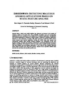
As mentioned above, we ran experiments on two envionment patterns, E1 and E2. In each case we ran experiments with different number of malicious nodes: 5, 10 and 15 respectively. During the online phase, we evaluated how quickly each of the reputation management schemes could detect the malicious nodes. In particular, we noted the number of data reporting intervals (iterations) taken by these mechanisms to detect the first and last erroneous nodes3 . We averaged the results over 10 random orderings of data reporting instances and have plotted the standard deviation (centered around the average value) as well as the minimum and the maximum iterations taken by these reputation schemes for the two problem sizes and two environments (see Figures 1, 2, 3, and 4). 3
The maximum iterations taken to detect the last erroneous node is the more important of the two metrics as it designates the time when all erroneous nodes have been detected
The maximum value of detection with first distribution 55
The minimum value of detection with first distribution 30
Max QL Max BR
50
26 number of cycles
45 number of cycles
Min QL Min BR
28
40 35 30 25
24 22 20 18 16
20
14
15
12
10
10 0
5
10
15
20
0
5
number of erroneous nodes
10
15
20
number of erroneous nodes
(a) Finding the maximum detection time for distribution 2 2 e−(x +y ) in eighty-five node network
(b) Finding the minimum detection time for distribution 2 2 e−(x +y ) in eighty-five node network
Figure 1: Maximum and minimum number of cycles required to detect compromised nodes by the Q-learning (QL) and RFSN (BR) approaches in environment E1 (n = 85).
The maximum value of detection with second distribution 350
The minimum value of detection with second distribution 90
Max QL Max BR
300
70
250
number of cycles
number of cycles
Min QL Min BR
80
200 150 100
60 50 40 30
50
20
0
10 0
5
10
15
20
0
number of erroneous nodes
(a) Finding the maximum detection time for distribution x+y in eighty-five node network 2
5
10
15
20
number of erroneous nodes
(b) Finding the minimum detection time for distribution x+y in eighty-five node network 2
Figure 2: Maximum and minimum number of cycles required to detect compromised nodes by the Q-learning (QL) and RFSN (BR) approaches in environment E1 (n = 85). All erroneous nodes were successfully identified for all scenarios and by both reputation management mechanisms, i.e., there were no false positives. Furthermore, there were no false negatives either, i.e., no non-erroneous leaf nodes were identified as faulty nodes. However, aggregators who had at least two faulty children were also detected to be faulty after an extended number of time intervals. This aspect is not plotted in the figures, and is of less importance because after faulty leaf-level sensor nodes would have been identified much earlier (we mention these here for the sake of completeness). Removing these would eliminate the need for eliminating their parents. We also note that the same mechanism used to identify faulty nodes at the leaf levels
of the hierarchy can be used to identify malicious nodes at higher levels.
3.4
Observations
From the results presented in Figures 1, 3, 2, and 4, we can make the following observations: • For every distribution the mean of minimum value of the cycle time for Q Learning based approach is less than that of RFSN based approach as shown in plots 1(b), 2(b), 3(b) and 4(b). This value remains between 12 to 15 iterations irrespective of the environment and number of erroneous nodes in the network (we have
The maximum value of detection with first distribution 65
The minimum value of detection with first distribution 26
Max QL Max BR
60
Min QL Min BR
24
50
number of cycles
number of cycles
55
45 40 35 30
22 20 18 16
25 14
20 15
12 0
2
4
6
8
10
0
2
number of erroneous nodes
4
6
8
10
number of erroneous nodes
(a) Finding the maximum detection time for distribution 2 2 e−(x +y ) in forty node network
(b) Finding the minimum detection time for distribution 2 2 e−(x +y ) in forty node network
Figure 3: Maximum and minimum number of cycles required to detect compromised nodes by the Q-learning (QL) and RFSN (BR) approaches in environment E2 (n = 40).
The maximum value of detection with second distribution 70
The minimum value of detection with second distribution 40
Max QL Max BR
35 number of cycles
number of cycles
60
Min QL Min BR
50 40 30 20
30 25 20 15
10
10 0
2
4
6
8
10
number of erroneous nodes
(a) Finding the maximum detection time for distribution x+y in forty node network 2
0
2
4
6
8
10
number of erroneous nodes
(b) Finding the minimum detection time for distribution x+y in forty node network 2
Figure 4: Maximum and minimum number of cycles required to detect compromised nodes by the Q-learning (QL) and RFSN (BR) approaches in environment E2 (n = 40). experimented with 15 and 7 faulty nodes at most for eighty five and forty node networks respectively). In case of the RFSN based approach and for n = 85, the mean of minimum iterations to identify a node in environment E1 is less than that in environment E2 when number of erroneous nodes are 15 (see Figures 1(b) and 2(b)). For n = 40, the minimum detection time for both the distributions are roughly equal (see Figures 3(b) and 4(b)). • For the time taken to detect the last erroneous node, the plots show that the means in case of the Q Learning based reputation management scheme is significantly
less than that of RFSN based approach irrespective of network size and the number of malicious nodes (see Figures 1(a), 2(a), 3(a) and 4(a)). With the RFSN based approach and for n = 85, the value for the mean of the maximum cycle time for environment E1 (see Figure 1(a)) is in the range of 25-40 iterations, which is significantly less than that required for environment E2 (see Figure 2(a)). The corresponding numbers lie range between 30-50 iterations for n = 40 (see Figures 3(a)and 4(a)). From the figures it is observed that Q-learning approach is faster in detecting the faulty or compromised nodes than
the RFSN based approach. Both maximum and minimum range of detection in Q-learning lies between 12 to 20 cycle time. The above results suggest that the neural net learning based approach can be combined with distributed reputation management schemes works efficiently in accurately detecting, i.e., without false positives and false negatives, anomalous sensor nodes within few data reporting intervals.
4. RELATED WORK Sensor networks, constrained with limited power supply, memory and computation ability, renders traditional security techniques inadequate and requires radically different power-aware solutions. Recently a lot of work has been done in securing sensor network applications like key establishment, secrecy, authentication, robustness to denialof-service attacks, secure routing and node capture. There has been some research in probabilistic key sharing to establish a secure path between neighboring nodes [9, 2]. From a large pool of symmetric keys, a random subset of keys is loaded to each sensor nodes, where the number of keys loaded per node depend on the desired probability of two nodes having a common key. Neighboring nodes can establish a secure path if they have a common key. This scheme has a scalability issue because it consumes memory to store keys which keeps increasing with growing network size and also presents the risk that the original key pool can be constructed if the attacker compromise sufficient number of nodes. Cryptography has been adopted as a standard solution to protect confidentiality, integrity and availability [11, 16, 10]. Faced with the limited power resource problem, symmetric key encryption is preferable over asymmetric versions. However SPINS [11] implements symmetric key cryptography with delayed key disclosure to achieve asymmetric key cryptography. SPINS incorporate both Secure Network Encryption Protocol (SNEP) which provides data confidentiality, authentication, integrity freshness and µTESLA [11] which provides authentication to broadcasts. Secure routing protocols have been used to maintain normal operation of sensor networks even when some nodes have been compromised [3, 8, 1]. Intrusion Tolerant routing in wireless Sensor Networks (INSENS) [3] works by creating routing tables at each node, thereby improving communication between nodes and the base station. INSENS tries to bypass malicious nodes and nullifies the effect of compromised nodes in the vicinity of malicious nodes. Most work on data aggregation [4, 7, 6, 13] assumes no node is malicious. SEF [15] and SDAP [14] has proposed a secure aggregation approach in presence of malicious nodes, which can detect and drop false reports. They use a pre key distribution technique along with cryptography to detect false data injection. However such a scheme has considerable overhead considering the resource constrains of sensor nodes. Sampling techniques has been used by Secure Information Aggregation in sensor networks (SIA) system [12] to calculate summary report even when a fraction of the nodes are malicious. The proposed technique in finding out the median, average, network size and maximum and minimum sensor reading would help the user verify the correctness of the data interactively. Existing literature on intrusion detection mechanisms in sensor networks use statistical approaches like outlier de-
tection schemes. These approaches assume that the entire sensor field has data sampled from the same distribution. Hence, any node that reports significant deviations from the average values reported by all nodes can be identified as faulty or compromised node. Such approaches that rely on a known distribution type and assumes uniform data values over the sensor field are limited in application. Sensor fields, often deployed from aerial vehicles can be spread over a relatively wide area, can have significant variation in the sensed data, e.g., temperatue, pressure, chemical concentrations, wind velocities, etc. can significantly vary even within relatively short physical distances. Our proposed approach does not make any prior assumption about uniformity or nature of data distribution over the sensor field but learns such patterns from reported data.
5.
CONCLUSION
In this paper, we have proposed a learning scheme to detect malicious nodes in a senor network that consistently or periodically report errors with small offsets to influence the aggregate data reported to the base station. Our approach uses a distributed reputation management mechanism that runs on internal levels of the sensor network organized as a hierarchy. Such an organization allows for creating a robust framework even if sizeable portions of the network is compromised. A malicious node is recognized when its reputation consistently deviates significantly from the other nodes. The other innovation in our work is the use of a learning based approach to model correlations between the data sensed at different nodes in the network. We propose a neighborhood based local approximation scheme for existing data patterns. Based on sensed data, we use an offline learning approach for developing predictors for each node given the data sensed by other nodes in its vicinity. Later, these learned models are used online to calculate deviations between the data reported by any node and the predicted value given the data reported by its neighbors. These deviations in successive data reporting periods are used by the parent of such a node in the hierarchy to update the reputation of the node. Nodes whose reputation plunges below a threshold are marked as faulty or compromised nodes. The combination of a neural network based offline Learning approach and a Q-learning or an RFSN based online repuation update scheme is experimentally demonstrated to be effective in identifying faulty node without any false positives and false negatives in the detection process. In our experiments, all erroneous nodes are successfully detected within a reasonable number of data reporting periods. The approach scales up nicely for different size sensor networks and is robust in the face of node failures and attacks even if as much as 25% of the nodes are corrupted. So, the system is robust against significant levels of collusion. We have tested it with a couple of data patterns that models significant deviations of the sensed parameters across the sensor field. In the future we intend to extend our work to incorporate the analysis of more sophisticated collusion, where malicious nodes may take turns to report high errors, and prevent malicious nodes from using false identities to report spurious, multiple false data. Other possible future directions include temporal correlations in the sensor field, e.g., tracking an object through the sensor field.
6. REFERENCES [1] B. Awerbuch, D. Holmer, and H. Rubens. Provably secure competitive routing against proactive byzantine adversaries via reinforcement learning. [2] H. Chan, A. Perrig, and D. Song. ” random key predistribution schemes for sensor networks”. In Security and Privacy: Proceedings of the 2003 Symposium, pages 197–213, May 2003. [3] J. Deng, R. Han, and S. Mishra. Insens: Intrusion-tolerant routing in wireless sensor networks, 2002. [4] A. Deshpande, S. Nath, P. B. Gibbons, and S. Seshan. Cache-and-query for wide area sensor databases. In SIGMOD ’03: Proceedings of the 2003 ACM SIGMOD international conference on Management of data, pages 503–514, New York, NY, USA, 2003. ACM Press. [5] S. Ganeriwal and M. B. Srivastava. Reputation-based framework for high integrity sensor networks. In SASN ’04: Proceedings of the 2nd ACM workshop on Security of ad hoc and sensor networks, pages 66–77, New York, NY, USA, 2004. ACM Press. [6] T. He, B. M. Blum, J. A. Stankovic, and T. Abdelzaher. Aida: Adaptive application-independent data aggregation in wireless sensor networks. Trans. on Embedded Computing Sys., 3(2):426–457, 2004. [7] C. Intanagonwiwat. Impact of network density on data aggregation in wireless sensor networks, Nov 2001. [8] C. Karlof and D. Wagner. Secure routing in wireless sensor networks: Attacks and countermeasures. Elsevier’s AdHoc Networks Journal, Special Issue on Sensor Network Applications and Protocols, 1(2–3):293–315, September 2003. [9] L.Eschenauer and V.D.Gligor. A key-management scheme for distributed sensor networks. In ”Proceedings of the 9th ACM conference on Computer and communications security”, pages 41–47, Nov 2002. [10] T. Park and K. G. Shin. Lisp: A lightweight security protocol for wireless sensor networks. Trans. on Embedded Computing Sys., 3(3):634–660, 2004. [11] A. Perrig, R. Szewczyk, J. D. Tygar, V. Wen, and D. E. Culler. Spins: security protocols for sensor networks. Wirel. Netw., 8(5):521–534, 2002. [12] B. Przydatek, D. Song, and A. Perrig. Sia: Secure information aggregation in sensor networks, 2003. [13] M. Sharifzadeh and C. Shahabi. Supporting spatial aggregation in sensor network databases. In GIS ’04: Proceedings of the 12th annual ACM international workshop on Geographic information systems, pages 166–175, New York, NY, USA, 2004. ACM Press. [14] Y. Yang, X. Wang, S. Zhu, and G. Cao. Sdap:: a secure hop-by-hop data aggregation protocol for sensor networks. In MobiHoc ’06: Proceedings of the 7th international symposium on Mobile ad hoc networking and computing, pages 356–367, New York, NY, USA, 2006. ACM Press. [15] F. Ye, H. Luo, S. Lu, and L. Zhang. Statistical en-route filtering of injected false data in sensor networks. IEEE Jounal on Selected Areas in Communications, Special Issue on Self-organizing Distributed Collaborative Sensor Networks,
23(4):839–850, April 2005. [16] S. Zhu, S. Setia, and S. Jajodia. Leap: efficient security mechanisms for large-scale distributed sensor networks. In CCS ’03: Proceedings of the 10th ACM conference on Computer and communications security, pages 62–72, New York, NY, USA, 2003. ACM Press.