Detecting Planar Homographies in an Image Pair Etienne Vincent and Robert Lagani`ere School of Information Technology and Engineering University of Ottawa Canada K1N 6N5
[email protected] [email protected]
Abstract This paper proposes an algorithm that detects planar homographies in uncalibrated image pairs. It then demonstrates how this plane identification method can be used as a first step in an image analysis process, when point matching between images is unreliable. The detection is performed using a RANSAC scheme based on the linear computation of the homography matrix elements using four points. Results are shown on real image pairs.
vision applications. An important contribution of this work, is to demonstrate that our algorithm can be used as a first step towards fundamental matrix estimation. Homographies were used to this end in [10] and [11], but we present a complete system for fundamental matrix estimation using planes, and demonstrate, its advantages. This paper is organized as follow: Section 2 reviews basic projective geometry concepts. Section 3 presents a proposed algorithm for planar homography detection, and Section 4 demonstrates that it should be used prior to fundamental matrix estimation.
1 Introduction
2 Projective Relations
Because of their abundance and simplicity, planes are used in several computer vision tasks such as autocalibration [14], reconstruction [7], visual measurement [2], and obstacle detection [8]. Their simplicity, results in that, under perspective projection, the transformation between a world plane and its corresponding image plane is projective linear, or a homography. These relations also hold between perspective views of a plane in different images. To benefit from the presence of planes, these structures must be detected. Some strategies have been proposed to do this, such as [11], where line segment groups or image pyramids are used. The approach presented here is based on RANSAC. Similar approaches have been used for homography detection in [8] to detect a ground plane, in [13] to detect a global homography, considered as a degenerate configuration of a fundamental matrix, and in other works. We will show how such a scheme can be implemented to detect many planar structures in a scene. In particular, we are interested in the case where matching is difficult, such as when the baseline is wide, or when repeated patterns are present. We will establish ways of improving the performance of the RANSAC algorithm under such conditions. Fundamental matrix estimation for uncalibrated image pairs, is an important, but sometimes difficult step in many
The fundamental matrix is a key concept in stereo vision. It represents the epipolar geometry of a system of two cameras. For each pair of corresponding points, represented by 3 × 1 homogeneous vectors (x, x0 ), the epipolar constraint is expressed as: x0T Fx = 0 (1) where F is the fundamental matrix, a 3 × 3 singular matrix with 7 DOF. A homography is a projective transformation represented as a nonsingular 3 × 3 matrix H. If x and x0 are images of the same world point, belonging to a plane, they are related by a matrix H corresponding to that plane: x0 = Hx
(2)
Since homogeneous coordinates are used, equality is up to an unknown scale factor. When several image points from a plane are available, H can be computed. For each pair of corresponding points, (2) gives two independent linear equations, when rewritten as: x0 × Hx = 0
(3)
Since the matrix H has 8 DOF, 4 point correspondences determine H.
Obviously, with non-perfect data, more points should be used. Then, H is estimated with a minimization scheme. This is done using: h = (h11 , h12 , h13 , h21 , h22 , h23 , h31 , h32 , h33 )T
(4)
N point correspondences give 2N linear constraints, using (3). This results in a system of the form Bh = 0. The following problem must then be solved: minh ||Bh||2 subject to ||h|| = 1
(b)
(c)
(d)
(5)
The solution being the eigenvector of BT B corresponding to the smallest eigenvalue. To obtain a more stable linear system, the coordinates of the point correspondence are normalized, as explained in [5], where a similar method is used to compute the fundamental matrix. Here, only algebraic quantities are minimized. It is preferable to minimizes a meaningfull geometric quantity. This is achieved using a non-linear minimization scheme. However, such a scheme requires an initial approximation, provided by the above method [2].
3 The Homography Detection Algorithm To detect planar homographies in uncalibrated image pairs, a RANSAC (Random Sample Consensus) scheme is used. The proposed algorithm is similar to the one presented in [1], where the fundamental matrix is estimated (see [9] for more on F estimation). There is however an important difference. In the case of F, all matches obey constraint (1), while with a homography, only image points of a common plane statisfy constraint (3). A different homography H must be detected for each visible plane.
3.1 The basic RANSAC Scheme 1. First corners are detected in both images [4, 6]. 2. Variance normalized correlation is applied between corners, and pairs with a sufficiently high correlation score are collected to form a set of candidate matches. 3. Four points are selected from the set of candidate matches, and a homography is computed using (3). 4. Pairs agreeing with the homography are selected. A pair (x, x0 ), is considered to agree with a homography H, if for some threshold ²: dist(Hx, x0 ) < ²
(a)
(6)
5. Steps 3 and 4 are repeated until a sufficient number of pairs are consistent with the computed homography.
Figure 1. An homography found using the algorithm. (a) and (b) The pair of images with the point matches agreeing with the homography. (c) Applying the homography to the right image. (d) Difference between the left image and (c).
6. Using all consistent correspondences, the homography is recomputed by solving (5). Fig. 1 shows a result of applying this algorithm to an image pair. When images are harder to match, because of a wide baseline, or repeated patterns, the correlation criteria must be relaxed, to ensure that enough valid matches from a plane are in the candidate match set. However, this results in a small proportion of valid matches in the candidate set, and a need for many iterations before finding a homography. This justifies the need for the strategies aiming at improving the efficiency of the process, that are introduced in the next sections.
3.2 Selecting the Four Points The way in which the four points are selected in step 3 of the algorithm, will influence the likelihood that they determine a valid homography. So far, the points are selected randomly from the set of candidate matches. To screen out degenerate configurations, the area between the selected points is used. The areas of the four triangles determined by the points is computed and the points are only considered for the next step if the areas are greater than a given threshold. This eliminates degenerate cases
where three of the points are colinear. It also avoids configurations where points lie too close to one another. Using this criteria, 50% of the selected four point configurations, in the image pair shown in Fig. 1 were eliminated. These were unlikely to produce valid homographies, so discarding them eliminated expensive computations. Another strategy is to select points lying on the same edges in an image. These are likely to belong to the same plane. However, points lying on the same edge are more likely to be colinear or to lie close to one another. The solution consists in choosing four points on two different edges. This increases the likelyhood of the points lying on the same plane, while generating fewer degenerate configurations. Similarly, two points lying on the same straight lines may be selected. This is especially advantageous when the disparity between two views becomes very significant. For example with the images shown in Fig. 5. this point selection heuristic gave, on average, a 37% improvement in the number of iterations needed to find a homography.
3.3 Using the Determinant To improve the efficiency of the algorithm, the determinant of the homography matrix can also be considered. If the determinant of a homography is close to zero, it corresponds to a degenerated case. If it is very large, the determinant of the matrix’s inverse (the inverse homography) will be close to zero. Consequently, homographies with determinants having an absolute value outside of a range [1/n, n], are discarded. This is advantageous since computing a determinant is less expensive then performing step 4. With the pair shown in Fig. 1, and n = 10, 51% of the preliminary homographies found, that satisfied the minimum area requirement, could be discarded.
(a)
(b)
Figure 2. Relaxing the distance threshold. (a) Applying the coarse approximation to the right image. (b) Applying the final approximation of the homography to the right image.
with the actual homography should be within this generous distance threshold of their expected positions. Among the putative compatible matches, a majority should be compatible with the real homography, thus, the computed homography should gravitate towards the valid one, as we iteratively recompute it. Once the homography has stabilized closer to its true value, the distance threshold can be tighten, as to only include the best matches in the computation. This technique, by allowing us to accept crude approximations of true homographies, and improving them to get the valid ones, can decrease by a factor of hundreds the number of iterations needed to detect a homography. Fig. 2 gives an example for which a crude approximation to a homography was found, with far fewer iterations (less then 1% of the iterations needed in Fig. 1). After improving this crude homography through relaxation of the distance threshold, the resulting homography also agreed with 38% more candidate matches then the one shown in Fig. 1.
3.5 Finding Subsequent Homographies 3.4 Relaxing the Distance Threshold It can be seen, during the homography estimation process, that several of the rejected homographies are close to valid ones. To reduce the number of iterations needed to find a homography cruder approximations of the homographies could be accepted, and then improved. We start with a generous distance threshold (the value of ² in equation (6)), such as 3 pixels, and a relatively low threshold for the number of points needed to be compatible with the homography. This allows a crude homography to be found relatively fast. To find the true homography, we iteratively recompute it using all matches compatible with it at that stage. This iterative process works well when the distance threshold is relaxed (increased up to 20 pixels). Since the computed homography is close to a valid one, most matches compatible
Image pairs often contain more than one plane. When a plane is identified, the matches compatible with it, can be removed from the candidate set. Incorrect matches having at least one of their points lying in a part of an image where the detected plane is visible, can also be eliminated. To decide which matches should be eliminated, the region of the image that agrees with the homography must be extracted. This is done by considering the result of applying the homography to one of the images in the pair. This transformed image should correspond almost exactly to the other one, in the area of the detected plane, while disagreeing in other regions. Thus, the absolute difference of the two images is computed, and thresholded. The obtained binary image is then cleaned up, using morphological operators. A closing using a small mask to eliminate the isolated errors in the plane
(a)
(b)
(c)
(d)
Figure 4. The number of trials required to find a planar homography in a scene compared to the number of trials required for weak calibration, both using RANSAC, as a function of the reliability of the match set used.
Figure 3. Finding a second homography (a) Difference between the left image and Fig. 2 d. (b) Regions in Fig. 2 c that agreed with the homography. (c) an (d) The point matches that agree with a second homography found after eliminating matches in the regions of (b) from the candidate matches set.
a good subset of matches in RANSAC is given by: p N
1 − (1 − (1 − ²out ) )
region, followed by an opening with a larger mask, to eliminate the isolated small areas falsely attached to the plane. All matches with a point in the identified region are discarded before attempting to find another homography. Fig. 3 illustrates the process of finding a second homography.
4 Estimation of the fundamental matrix An important application of the planar homography detection algorithm, would be in the estimation of F (weak calibration). The fundamental matrix can be estimated using two or more homographies [10, 11]. The estimation is performed using matches compatible with the homographies, or directly from the homography matrices. In this latter case, the following relation between F and H is used: HT F + FT H = 0
(7)
The estimation of F using homographies may be less accurate then a direct approach, but can serve as a starting point to a better estimation. Let us now compare the problem of planar homography detection using RANSAC, to direct fundamental matrix estimation using RANSAC, in the context of noisy data. The theoretical expression of the probability of selecting
(8)
where p is the number of matches needed to compute a solution (4 for H, 8 for F), ²out is the proportion of the matches that are not compatible with the homography or fundamental matrix, and N the number of iterations performed. In the case of homography detection, ²out is larger since not all good matches lie on a single plane. We will make the reasonable assumption that half of the good matches are compatible with some homography. The ratio between the number of iterations that would be necessary to perform the two tasks with the same probability of success can be computed from (8): NH log (1 − r8 ) = 4 NF log (1 − ( 1+r 2 ) )
(9)
H where N NF is the ratio of the number of trials needed to compute H to the number of trials needed to compute F, and r is the proportion of valid matches in the data set. H Fig. 4 shows the theoretical ratio N NF , as a function of the proportion of the candidate matches that are valid. It can be noticed that it is far easier to find a planar homography than to perform calibration, when using very noisy data. Such noisy candidate sets occure, when an image pair has a wide baseline, or contains repeated patterns. An example where it was much less expensive to use homography detection, prior to fundamental matrix estimation is given in the next section.
Dept of Eng. Science, University of Oxford, 1996. [2] A. Criminisi, I. Reid, A. Zisserman, A Plane Measuring Device, Image and Vision Computing, Vol. 17, 625-634, 1999.
(a)
(b)
Figure 5. An image pair, and the matches agreeing with a detected planar homography.
5 Additional Experimental Results Fig. 5 shows a homography that was identified in an image pair where the perspective difference between the images is significant. The four points were selected so that pairs of points lied on two different automatically dected lines, as described in subsection 3.2. The algorithm succeeded in finding a homography despite the wide baseline. Fig. 6 shows three homographies that were identified in an image pair. The candidate match set was constructed using a Harris corner detector [4], and variance normalized correlation. This set contained only about 15% of valid matches, in part because of the repeated window patterns. The homographies were obtained after 1071, 2605, and 677 iterations respectively. The fundamental matrix was also computed directly from this candidate set with a RANSAC scheme, using the implementation [12], and required 24500 iterations. Thus, it was greatly advantageous, in this image pair, to first detect the homographies. The fundamental matrix could easily be approximated using the candidate pairs that agreed with the homographies.
6 Conclusion We have presented an algorithm for the detection of planar homographies in image pairs. We have demonstrated that by using appropriate strategies, the algorithm can effectively detect the visible planar structures even when the available match set is unreliable. This robustness makes the algorithm attractive as a first step in vision processes. In particular, we have shown that it could be used with great advantage towards weak calibration when the set of matches is noisy, and planes are expected to be present.
References [1] P. Beardsley, P. Torr, A. Zisserman, 3D Model Acquisition from Extended Image Sequences, Technical report,
[3] O. Faugeras, Q. Luong, S. Maybank, Camera selfcalibration: Theory and experiments, Proc. ECCV, pp. 321-334, 1992. [4] C. Harris, M. Stephens, A Combined Corner and Edge Detector, Alvey Vision Conf., pp. 147-151, 1988. [5] R. Hartley. In Defense of the Eight-Point Algorithm, PAMI, Vol. 19, pp. 133-135, 1997. [6] R. Lagani`ere, A Morphological Operator for Corner Detection, Pattern Recognition, Vol. 31, pp. 1643-1652, 1998. [7] D. Liebowitz, A. Criminisi, A. Zisserman, Creating Architectural Models from Images, Proc. EuroGraphics, 1999. [8] M. Lourakis, S. Orphanoudakis, Visual Detection of Obstacles Assuming a Locally Planar Ground, Proc. ACCV, pp. 527-534 1998. [9] Q.-T. Luong, R. Deriche, O. Faugeras, T. Papadopoulo, On determining the Fundamental matrix: analysis of different methods and experimental results, Technical Report, INRIA, 1993. [10] Q.-T. Luong, O. Faugeras, Determining the Fundamental matrix with planes: unstability and new algorithms, Proc. CVPR, pp. 489-494, 1993. [11] P. Pritchett, A. Zisserman, Matching and Reconstruction from Widely Separated Views, 3D Structure from Multiple Images of Large-Scale Environments, LNCS 1506, Springer-Verlag, 1998. [12] G. Roth, A. Whitehead, Using Projective vision to find Camera Positions in an Image Sequence, VI, pp.225232, 2000. [13] P. Torr, A. Zisserman, S. Maybank, Robust Detection of Degenerate Configurations for the Fundamental Matrix, Computer Vision and Image Understanding, Vol. 71, pp. 312-333, 1998. [14] B. Triggs, Autocalibration from Planar Scenes, Proc. ECCV, pp. 89-105, 1998.
(a)
(b)
(c)
(d)
(e)
(f)
Figure 6. Three homographies found using our RANSAC-like algorithm on an image pair. (a) and (b) The point matches that agree with a first homography. (c) and (d) The point matches that agree with a second homography. (e) and (f) The point matches that agree with a third homography.