an algorithm for detecting and labeling drum events in ... - CiteSeerX

AN ALGORITHM FOR DETECTING AND LABELING DRUM EVENTS IN POLYPHONIC MUSIC Koen Tanghe1, Sven Degroeve2, Bernard De Baets2 1 IPEM, Department of Musicology, Ghent University, Blandijnberg 2, 9000 Ghent, Belgium 2

[email protected]

Department of Applied Mathematics, Biometrics and Process Control, Ghent University

ABSTRACT This document describes an algorithm that tries to locate and label drum events in polyphonic musical audio. The three main parts of the algorithm are described in detail and an overview of the developed applications is given. Finally, the results of an evaluation performed in the context of the ISMIR2005 MIREX “contest” [1] are reported. Keywords: drum detection, onset detection, feature extraction, support vector machines, audio-to-MIDI

1 INTRODUCTION This research was started in the context of the Musical Audio Mining (MAMI) project [2]. In order to query databases of musical audio based on the musical content itself (which is what this project is about), one needs to have descriptions of that musical content. Transcribing the drums in a musical piece is therefore one possible way to obtain such a description. Obtaining melodic information is another one, but since drum sounds are very important in many popular music genres nowadays, we thought it would also be interesting to focus on this aspect of the music. Also, drum detection research has not gained as much attention over the last decades as melody extraction research, which makes it an even more interesting topic to study. Our earlier studies ([3],[4]) mainly dealt with only one particular aspect of the drum detection process or with drum detection in a more restricted environment, whereas this document describes the final overall system that was also used for the audio drum detection track of the ISMIR2005 MIREX “contest” and works on “full” CD-quality music. The algorithm we developed can be categorized as a feature-based classification method. The algorithm used by Gillet and Richard [5] which also entered the MIREX “contest” is similar to our method in that it also performs onset detection, feature extraction and feature vector classification using Support Vector Machines. However, their method performs a band-wise noise subspace projection before the onset detection and feature extraction stages and it also uses an extra adaptation stage at the end that builds a “localized” model per audio excerpt, which is then used to obtain a more specialized classification for that particular fragment.

2 ALGORITHM DESCRIPTION 2.1 Overall scheme This drum detection algorithm has an architecture consisting of three main parts, which are shown in figure 1. The onset detection is the first stage. It locates moments in time where drum events might be present. The second stage is the feature extraction stage where features are extracted from the audio around the detected onsets. And finally the classification stage makes a decision for each onset (based on the extracted audio features) about which type of event is present at that location (drum event or not, and if so, which type of drum event). Each of these three stages is specified on the following pages. audio signal

onset detection

feature extraction

feature classification label Figure 1: Overall architecture of the drum detection module.

2.2 Training and application phase As we are using a supervised machine learning method, the overall methodology is actually split up in two phases: a “training phase” and an “application phase”. In order to use the drum detection algorithm on unseen audio in the application phase, it must first be trained during a training phase, in which it is fed with audio for which the drum events are known in advance. In this training phase, the user supplies pairs of sound files and corresponding MIDI files which contain a symbolic representation of the drum events that can be heard in the sound file. This means that for each relevant drum event in the sound file, there is a MIDI note

on message at that moment and for that specific drum type on channel 10 in the MIDI file. The drum types represent abstract categories of drum sounds such as bass drums, snare drums etc… Each of these drum types gets a label (BD, SD, …) and there may be multiple MIDI note numbers that correspond to the same drum type. Obtaining the training audio and MIDI files is usually accomplished using two common methods. The first starts from an existing MIDI file, usually either a full MIDI file as can be found on the Internet, or a MIDI file from a music production project (programmed drums, or drums recorded on an electronic drum kit). The corresponding audio file is then obtained by recording the audio output while playing back the MIDI file through various synthesizer instruments, possibly together with audio tracks containing additional voice or guitar recordings. The second method works the other way around and starts from the audio file, which is manually annotated using a combination of MIDI drum performance recording and MIDI drum track editing. This can be done in a sequencer program where the audio file is put on an audio track, and a MIDI track is filled in by the annotator who tries to imitate what he hears by placing drum events on that MIDI track [8]. While being more timeconsuming than the first method, this method can be applied to music for which the MIDI drum events are not readily available and allows us to work with music files that are of the same realistic quality as the ones the algorithm will operate on in the application phase.

2.3.3 Calculating amplitude changes For each of the N frequency bands, a weighted sum of the differences between the current amplitude level and that of the recent past is calculated. More recent values have a higher importance than older ones. The N outputs of the Mel filter bank are also processed by an envelope follower, which roughly follows the overall shape of the amplitude fluctuations over a longer period of time. By dividing the weighted differences by the corresponding envelope follower outputs, we obtain a relative difference value for each frequency band, which is a measure for the amount of energy change in that band. Figure 2 shows the processing scheme up to this point.

audio signal 1

STFT NB

N

circular buffer N

weighted difference N N

envelope follower

Since the classification stage should be able to distinguish between drum events and non-drum events, we would rather have the onset detector detect too many onsets than too few. If the classifier is good enough, it should be able to throw out the non-drum events. Of course, there are limits: in the extreme case we could just feed the whole continuous stream of audio features to the classifier instead of first doing some onset detection, but that is very inefficient. And it might not even work well either: multiple drum events would most probably be detected around onset locations at the feature vector sample rate, so a mechanism to extract the exact event location from these multiple events would still be needed after all. Hence, the use of an onset detection stage was chosen. 2.3.2 Splitting up the signal in different frequency bands First of all, the input signal is routed through a windowed short term Fourier transform (of which we only use the amplitudes) and a triangular shaped Mel scale filter bank to obtain a multi-band spectral representation of the audio signal at a reduced sampling rate. The results for each frame step are stored in a circular buffer for consultation later on.

/ N

2.3 Onset detection 2.3.1 Introduction

mel filterbank

N

relative differences Figure 2: Calculation of amplitude changes.

2.3.4 Making decisions Method 1 In this method, the relative differences in each frequency band are summed together and divided by the number of bands. This one-dimensional stream of summed relative differences is then sent through a module that decides whether an onset occurs at this moment or not. An explanation of the heuristics on which this decision is based can be found below. The (simple) scheme for this decision method is shown in figure 3 on the left. Method 2 In this method, the relative differences in each frequency band are first sent through a peak detector that just checks if a local maximum has occurred in any of the bands. If this is the case, an additional check is done to see if that maximum is strong enough (higher than a threshold value) to be kept. For each time step, this results in a Boolean vector for which a "true" means that a strong peak occurred in the corresponding frequency band. Just like in method 1, this (now multidimensional)

result is then sent through a module that decides whether or not an onset really occurred. See figure 3 for the scheme of this method. relative differences

relative differences

N

peak detector

N

normalized sum

N

thresholding

1

heuristic grouping peak detector b oo l

trigger

N

heuristic grouping peak detector b oo l

trigger Figure 3: Making onset decisions (methods 1 and 2).

Heuristic grouping peak detector This processing block is rather important because it needs to make the final decision about whether or not an onset occurred, based on the recent history of relevant peaks (in different bands for method 2). Because peaks in different frequency bands often do not occur at the exact same moment in time, and do not always lead to a single overall peak, we need to use some heuristics in order to make a more robust decision. The processing scheme is shown in figure 4. input vector n

sum 1

1

peak detector

circular buffer

b oo l

1

sum over grouping interval

check peak is above threshold and level was below hysteresis

1

circular buffer 1

b oo l

circular buffer

b oo l

b oo l

check value at minIOT in past false

true

check for more recent higher peaks b ool

trigger

Figure 4: Heuristic grouping peak detector processing scheme.

First, all elements of the input vector are summed together and the sum is stored in a circular buffer (in case

of a Boolean vector, 1 is used for "true" and 0 for "false"). Then the sum of these sums over a certain period in the past is calculated and stored in another circular buffer. For method 2, this effectively comes down to counting the number of relevant peaks over all frequency bands in the last x milliseconds. This stream of values is sent through a peak detector that outputs "true" if a local maximum is reached or "false" if not. If a local maximum has occurred, we check if the peak value is above a certain threshold, and if the level has up to now been below a certain hysteresis level. This hysteresis is added to alleviate the well-known problem encountered with simple thresholding where small fluctuations around the threshold level may cause multiple on/off triggers. The result is stored in a circular buffer (the "peak candidate buffer"). Up to here, we have been dealing with a single possible new peak candidate. From here on, we will be dealing with the set of buffered peak candidates and try to find out if a peak at the end of the buffer (which occurred some time ago) is indeed a final peak or not. To do that, we extract the oldest value from the "peak candidate buffer" and check its value. If this is "false", we output "false" and hence decide "no onset" at that moment in time (note that this moment lays in the past, so we have a delay here). If this is "true", we check if there are more recent peaks that are higher than the one we are considering. If this is the case, we decide "no onset" at that moment in time. If this is not the case, we set all more recent peaks to "false" (thus eliminating them as possible future onsets), and decide "onset" at that moment in time. To summarize: the sum of all channels over a specified grouping period is calculated only peaks in this sum higher than a threshold value are considered after a detected peak, the calculated sum must decrease below a certain hysteresis level before a new peak can be detected a minimum time interval between two successive peaks is specified and within this period, the highest peak is withheld So as the final output of the onset detector, we get a continuous stream of Boolean values where a "true" means that an onset has occurred a fixed amount of time in the past (this fixed delay is on the order of 40 to 100 ms, adjustable by the user). 2.4 Feature extraction 2.4.1 Introduction We assume that a fixed amount of audio data following a potential drum onset (detected in the first stage) contains enough information necessary to make a valid decision in the last (classification) stage. The feature extraction stage reduces the raw audio samples from this context to a more compact and more meaningful representation of the audio content, by calculating some properties that are

thought to be relevant for discriminating different types of percussive sounds. The module receives a continuous stream of audio samples and always performs some light processing on this stream (no matter whether an onset was detected or not). This only involves DC-blocking, very low level noise addition (to avoid numerical instability problems) and 3 band filtering (if needed for the requested features). Results are stored in circular buffers that are big enough to hold at least a number of values corresponding to the context length (CL) over which features should be extracted (specified as a duration in seconds). At any time, the module can be asked to extract a feature vector, which is calculated over the buffered data and hence corresponds to a segment of length CL and starting at now - CL. This means that if at a certain time T an onset is reported by the onset detection stage, the request to calculate a feature vector should be delayed by CL so that the segment that is used when the calculations are performed effectively contains all samples over a duration of CL starting at T and ending at T + CL (see figure 5). start

bands. The filters are simple Butterworth filters and were designed using Matlab's buttord and butter functions (the amplitude response of these filters is shown in figure 7): fs = 44100; [Ord,Wn] = buttord([49 50]/(fs/2),[0.01 2000]/(fs/2),0.01,62); [B{1},A{1}] = butter(Ord,Wn); [Ord,Wn] = buttord([200 201]/(fs/2),[1 1300]/(fs/2),0.01,20); [B{2},A{2}] = butter(Ord,Wn); [Ord,Wn] = buttord([5100 16300]/(fs/2),[65 22000]/(fs/2),0.05,60); [B{3},A{3}] = butter(Ord,Wn);

For each of the three filtered signals, RMS is again calculated as was done for the overall RMS, yielding RMSb1, RMSb2 and RMSb3: one RMS value for each band.

end CL past

future now T + CL

last onset T

Figure 5: Calculation of features over a fixed context.

All N features are represented by one or more real values, and are combined into a single feature vector, so for each onset from stage 1, there is a feature vector of length N corresponding to an audio segment starting at the onset time and ending at the onset time + CL. The extracted audio features are explained in detail below.

Figure 6: Accumulated amplitide spectra for different drum types.

2.4.2 Extracted features • RMS in the overall signal This is simply a basic measure for the overall sound level of the audio and is calculated as the root-mean square value of all samples in the segment, in dB. Here N is the number of samples in the segment, and xi is the i -th sample of the segment: N −1

RMS = 20.log10

∑x i =0

2

i

N

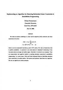
• RMS in 3 frequency bands When inspecting the accumulated spectra of hundreds of bass drums, snare drums and hihats, it can be seen that the spectral energy distributions of these different sounds are located in more or less distinct frequency bands, although not completely separated (see figure 6). Hence we divided the spectrum into three frequency bands and computed energy-related features over these

Figure 7: Amplitude response of the three drum filters.

• RMS per band relative to overall RMS Since the contribution of the 3 frequency bands to the overall sound level can be more interesting than the absolute levels, we also calculate relative levels as follows: RMSb1Rel = RMSb1 - RMS RMSb2Rel = RMSb2 - RMS RMSb3Rel = RMSb3 - RMS

• RMS per band relative to RMS of other bands The differences in sound level between the different frequency bands are also calculated: RMSbRelComb12 = RMSb1 - RMSb2 RMSbRelComb13 = RMSb1 - RMSb3 RMSbRelComb23 = RMSb2 - RMSb3 • zero-crossing rate This feature reports the number of times the signal changes sign per second. To avoid obtaining high values only due to noise, we use a zero-tolerance level of -60 dB, which means that only zero-crossings that go from -ZT to +ZT (or vice versa) are taken into account as genuine zero crossings (ZT = 0.001 in this case). • crest factor The crest factor is calculated as the ratio between the maximum absolute value of the signal and its RMS value. The crest factor of a musical signal is known to be much higher than for a speech signal. CrestFactor =

max ( x ) RMS ( x)

• temporal centroid The temporal centroid is calculated as the centre of gravity of the distribution of the power values of the samples in the segment. The lower this is, the more energy is located at the beginning of the segment (and vice versa). N −1

TempCentroid =

∑ i.x i =0 N −1

2 i

∑x i =0

2 i

• spectral centroid This is calculated as the centre of gravity of the power spectrum. Roughly speaking, the lower this is, the more energy is located in the lower frequency components (and vice versa). NF −1

SpecCentroid =

∑

f i .P ( f i )

i =0 NF −1

∑ P( f ) i

i =0

• spectral kurtosis Spectral kurtosis is calculated as the fourth order moment of the power spectrum, offset by -3. It says something about the size of the tails of the distribution of the amplitude spectrum values. Distributions with relatively large tails have positive kurtosis, distributions with small tails have negative kurtosis, and normal distributions have zero kurtosis. In the following formula, µ = mean and σ = standard deviation: NF −1

SpecKurtosis =

∑ ( P( f ) − µ ) i =0

i

N .σ

4

4

−3

• spectral skewness Spectral skewness is calculated as the third order moment of the power spectrum. It says something about the

symmetry of the distribution of the amplitude spectrum values. A value of zero means that the distribution is symmetric and a positive (respectively negative) value means that the distribution has a tail at the higher (respectively lower) values. NF −1

SpecSkewness =

∑ ( P( f ) − µ )

3

i

i =0

N .σ 3

• spectral rolloff The spectral rolloff determines the lowest frequency at which the accumulated sum of all lower frequency power spectrum values reaches a certain fraction of the total sum of the power spectrum. We used R = 0.85 as rolloff fraction. SpecRolloff =  min  f j 



NF −1

j

∑ P ( f ) ≥ R. ∑ P ( f ) i

i =0

i

i =0



• spectral flatness The spectral flatness is defined as the ratio of the geometric mean to the arithmetic mean of the power spectrum. It is a measure of the flatness of the spectrum. Values near 1 are obtained for a flat spectrum and values near 0 for a peaky spectrum. N −1

N

SpecFlatness =

∏ P( f )

1 N

i =0 N −1

i

∑ P( f ) i =0

i

• Mel frequency cepstral coefficients and deltas MFCCs and their derivatives are a much-used lowdimensional representation of the spectral content of an audio signal (especially in speech-processing contexts). We calculate MFCCs using the following FFT-based method: - apply window to signal fragment (audio frame) - get normalized FFT magnitudes (squaring is optional) - apply triangular shaped Mel filter bank to FFT magnitudes and sum (different FFT bin weightings for each filter) - apply log operator to filter outputs (optional) - apply DCT (discrete cosine transform) If we consider the MFCCs as zero order deltas, then the higher order deltas are derived from the lower order ones by applying one of the calculations below: - deltas ( WS = window size in samples): WS

di =

∑ d .( c d =1

i+d

− ci − d )

WS

2.∑ d 2 d =1

- simple deltas ( d = fixed window size in samples): di =

ci + d − ci − d 2.d

MFCCs and their higher order deltas are calculated over a sliding frame with a fixed width (we use 20 ms by default) moving from start to end of the segment using a specific frame step (we use 10 ms by default).

We then calculate the mean and standard deviation for each of the coefficients over all frames (the whole segment) and these values are stored in the feature vector. By default, we use a Mel filter bank of 20 normalized filters covering the entire frequency range; we use the FFT amplitude spectrum (no squaring), apply a log operator after the filter bank and only keep the first 12 coefficients. For the derivatives, we usually calculate only the first and second order deltas (not simple deltas), with a delta window size of 2. So, with these default settings, this gives us a 12*3*2 = 72 values that are added to the feature vector. Some work on optimizing some of these MFCC parameters together with the context length has been done in [6]. 2.5 Feature vector classification This stage applies a classification model computed by the Support Vector Machine (SVM) inductive learning method. The SVM is a data driven method that constructs a classifier that separates the data in a training set with low error and large margin [7]. The SVMs are used to make a decision about which drum types the extracted feature vectors represent (if any). N binary classifiers are used (where N = number of classes) since different drum classes can (and will) occur at the same time. Both linear and Gaussian kernels have been used successfully, but the Gaussian ones consume more CPU power (which might be important when using the algorithm in a realtime context). The free parameters for the SVM models (one for the linear kernel, two for the Gaussian ones) are optimized in the training phase using cross-validation over a prelabelled set of feature vectors extracted from annotated audio files. These features are extracted around the onset times found in the annotations and are thus only dependent on the feature extraction parameters. The training data is scaled to [-1,1] (scaling factors are stored in a “scale file”) and SVM models are created from this scaled data (each model is stored in a “model file”). In the application phase, the classification is then done for each drum type by first scaling each new test vector using the stored scaling factors and then applying the SVMs on each test vector using the stored models. 2.6 Streaming, causality and delays This algorithm operates in a streaming way, which allows us to process both very big audio files and neverending live audio streams. This implies that the audio must be processed as it comes in, so we can't wait to start processing until after we have read all audio samples (in fact, there is no such thing as "all audio samples" when dealing with streams). This also means that things like "normalizing by the maximum" are not possible and need to be replaced by functionality working on the recent past stored in circular buffers. This usually makes the algorithms more adaptive to variations in the audio, but also introduces a certain amount of "adaptation time" and a (preferably small) delay. This delay is inherent to

all causal audio analysis systems: you can’t make a decision about something until after you have heard (at least some part of) it. We did not yet try to incorporate methods to make predictions about the future based upon analysis results from the (recent) past. Both the onset detection stage and the feature extraction stage require a “working memory“ of several tens of milliseconds. However, the overall delay of the drum detection algorithm is determined by the maximum of these two delays, rather than by the sum, as can be seen in figure 8. Typical values are 80 ms for the feature extraction (depends on the context length) and 105 ms for the onset detection (depends mainly on the parameters of the STFT and the heuristic grouping peak detection). Extra internal buffering is done to synchronize the onset detection and feature extraction streams. FE::GetFeatureVector

OD::Process

FEDelay past ODDelay

onset

future

now

ODDelay > FEDelay total delay = ODDelay FE needs extra buffering (amount = ODDelay - FEDelay)

OD::Process

FE::GetFeatureVector

FEDelay past onset

ODDelay

future

now

ODDelay < FEDelay total delay = FEDelay OD needs extra buffering (amount = FEDelay - ODDelay)

Figure 8: Onset detection and feature extraction delays.

3 DEVELOPED APPLICATIONS 3.1 Implementation The algorithm and all of its components are implemented in standard C++ and run on Windows and Linux. Although the code is currently not optimized (both algorithmically and technically), the complete algorithm does work faster than real-time (with file output for intermediate results turned off): 16.3% of real-time on an Intel Pentium 4, 3.2 GHz and 33.9% of real-time on an AMD Athlon XP 1700+, 1.5 GHz. Several third party libraries are being used: libsndfile for sound file I/O [10], libsvm for the SVM functionality [11], Div's Standard MIDI File API for MIDI file I/O [12] and FFTReal for the fast Fourier transforms [13]. All these libraries have a license that facilitates commercial use, in case this would ever be desired. All software mentioned below can be found on the public section of the MAMI project website [2].

3.2 Console applications

4 EVALUATION AND RESULTS

In order to make the various stages of the drum detection algorithm usable for non-programmers and for working with a batch of audio files, several console applications were developed that can be run from the command line. These are the binaries that were submitted to the MIREX 2005 contest for evaluation. They are all file-based (inputs and outputs are sound files, MIDI files or text files) and can be used either separately or chained together in a batch file or script. Apart from the applications for the three main stages of the drum detection, there are also a few extra applications for extracting drum events from MIDI files, for converting between different text-based annotation file formats, for preparing the data files for the SVM training and for rendering the detected (or annotated) events to an audio file for aural feedback. See figure 9 for an overview. Training phase input

sound file

MIDI file

Application phase input

DrumEventExtractionFromMIDICA

sound file

DrumOnsetDetectionCA

occurrence file

onset file

DrumFeatureExtractionCA

feature file

DrumSVMDataFilePreparationCA

DrumFeatureClassificationSVMCA

output

svm-scale

occurrence file

Resynthesis

scaled SVM data files occurrence file

drum sound files

svm-train DrumDetectionResynthesisCA output

SVM scale files

For the MIREX 2005 evaluation, three data sets of annotated audio files were available. The data sets were named after their providers: CD (Christian Dittmar from Fraunhofer IDMT), MG (Masataka Goto from AIST [9]) and KT (Koen Tanghe from Ghent University [8]). In short, all audio files are mono WAV PCM files at 44.1 kHz, having a duration varying from 30 s (music fragments, KT and CD set) to several minutes (complete songs, MG set). All audio files were annotated for three drum types: bass drum (BD), snare drum (SD) and hihats (HH). Out of the complete data set, 23 sound files (4 from the CD set, 9 from the KT set and 10 from the MG set) with their corresponding annotation files were chosen by the organizers as the development set, and these files could be used by the participants as they pleased. The rest of the data is kept as “test data” for the actual evaluations. More details can be found on the MIREX web pages [1]. 4.2 Evaluation and results

DrumFeatureExtractionCA

feature file

SVM data files

4.1 Development data and test data

SVM model files

sound file

Figure 9: Overview of the developed console applications.

3.3 Audio-to-MIDI application All stages of the drum detection application phase are also combined into a single monolithic console application that takes in a mono sound file and produces a MIDI file containing the detected drum events. Algorithm settings can be specified using a parameter file, and the mapping of the considered drum types to MIDI note numbers is done through a MIDI drum label map. The program can also process a list of sound files in one go and an option to output ASCII drum event list files is provided as well (which might be easier to import in some programs). Parameter, model and scale files used for the MIREX 2005 contest are provided as defaults. 3.4 Library Finally, we are working on a C/C++ library to allow third parties to incorporate the streaming drum detection functionality in their own software.

The evaluation of the submitted algorithms is done by comparing the list of detected drum events with the list of annotated events (the ground truth). An F-measure score (with equal importance to precision and recall) is calculated for each drum type, resulting in three Fmeasure scores and their average score. Only events detected within a range of 30 ms around the ground truth events times can be accepted as correct. To have an idea about the processing power each algorithm requires, a speed measure is calculated as well. Overall results for our algorithm run on a 3 GHz Intel Pentium 4 machine running Windows XP are shown in table 1. Tables with separate results for each of the three data sets and results for the other participants’ algorithms can be found on the MIREX web pages [1]. Submission Average Classification F-measure Overall Onset Precision % Overall Onset Recall % Overall Onset F-measure BD Average F-measure HH Average F-measure SD Average F-measure Runtime (s) Machine

3 0.611

4 0.609

1 0.599

63.30 71.19 0.67 0.688 0.601 0.555 1337 Y

62.57 71.09 0.666 0.686 0.59 0.562 1342 Y

60.02 72.45 0.657 0.677 0.588 0.542 1350 Y

Table 1: MIREX 2005 evaluation results.

We originally submitted 4 versions of our algorithm, of which only 3 were retained by the organizers for the evaluation. Version 1 uses RBF kernels for the SVM models and onset detector parameters that had been previously optimized on the whole KT data set only (no data from other MIREX participants) [8]. Version 3 is

the same as version 1, but uses a minimum inter-onset time of 100 ms (instead of 79 ms). Version 4 is the same as version 1 but uses onset detector parameters that were optimized on the MIREX development data set only. All our versions performed equally well and obtained a main score of around 0.61 (for comparison: the main score for the best algorithm was 0.67). Best results with our algorithm were obtained for bass drums, followed by hihats and then snare drums. A remarkable fact is that all participants’ algorithms (save one) have their highest scores for the MG data set, followed by the CD data set and then the KT data set (always lowest).

5 FUTURE WORK One of the items near the top of our “to do” list is setting up an easy way to perform the training phase. Whereas the application phase functionality has been wrapped in a set of ready-to-use console applications and a global audio-to-MIDI application, the training phase is currently implemented as a collection of Perl scripts that find appropriate parameters automatically using standard cross-validation techniques and a set of Matlab functions for optimizing the onset detection parameters. A single application where one specifies a set of audio files, the corresponding set of MIDI annotation files and a drum label map, would allow a user to adapt the system to a particular type or style of music, which will always work better than using a very generic model. For offline use on sets of audio files, we would like to investigate to what extend building “localized models” on a file-per-file basis improves the performance. The algorithm also needs to be properly evaluated with more than three drum types and the efficiency should be further improved by optimizing both the algorithm itself and its implementation. Finally, we would also like to investigate if and how this work could be used in music production systems and real-time interactive multimedia systems, where robustness, usability issues and processing latency play an important role.

6 CONCLUSIONS This paper presented the details of a real-time streaming drum detection algorithm and its three main processing stages, operating on “full” CD-quality music. Results of an evaluation for three drum types performed in the context of an international conference were reported, where the algorithm was ranked second best (out of five). The drum detection functionality is made available as a set of console applications, an overall audio-to-MIDI application and a C/C++ library, which can all be downloaded from the MAMI project website [2].

ACKNOWLEDGEMENTS This work was done in the context of the “Musical Audio Mining” (MAMI) project, which is funded by the Flemish Institute for the Promotion of Scientific and Technological Research in Industry.

REFERENCES [1] Music Information Retrieval Evaluation eXchange (MIREX), http://www.music-ir.org/mirexwiki [2] Musical Audio Mining (MAMI), Ghent University, Belgium, http://www.ipem.ugent.be/MAMI [3] D. Van Steelant, K. Tanghe, S. Degroeve, et al. “Classification of Percussive Sounds Using Support Vector Machines”, Proceedings of Benelearn 2004, Brussels, Belgium, 2004 [4] D. Van Steelant, K. Tanghe, S. Degroeve, et al. “Support Vector Machines for Bass and Snare Drum Recognition”, Proceedings of GfKl 2004, Dortmund, Germany, 2004 [5] O. Gillet and G. Richard “Drum track transcription of polyphonic music using noise subspace projection”, Proceedings of ISMIR 2005, London, UK, 2005 [6] S. Degroeve, K. Tanghe, et al. “A Simulated Annealing Optimization of Audio Features for Drum Classification”, Proceedings of ISMIR 2005, London, UK, 2005 [7] V. N. Vapnik, “The Nature of Statistical Learning Theory”, Springer, 1995 [8] K. Tanghe, M. Lesaffre, S. Degroeve, et al. “Collecting ground truth annotations for drum detection in polyphonic music”, Proceedings of ISMIR 2005, London, UK, 2005 [9] M. Goto, “Development of the RWC Music Database”, Proceedings of ICASSP 2004, Montreal, Canada, 2004 [10] E. de Castro Lopo, “libsndfile, a C library for reading and writing files containing sampled sound”, http://www.zip.com.au/~erikd/libsndfile [11] C.-C. Chang and C.-J. Lin “libsvm, a library for Support Vector Machines”, http://www.csie.ntu.edu.tw/~cjlin/libsvm [12] D. G. Slomin “Div's Standard MIDI File API”, http://www.sreal.com:8000/~div/midi-utilities-forwindows [13] L. De Soras “FFTReal, a C++ class for computing the FFT of vectors of real numbers and their inverse FFT”, http://ldesoras.free.fr/prod.html