Detection and Localization in Colored Noise via Generalized Least ...

IEEE TRANSACTIONS ON SIGNAL PROCESSING, VOL. 44, NO. 7, JULY 1996

1734

Detection and Localization in Colored Noise via Generalized Least Squares Mati Wax, Fellow, IEEE, Jacob Sheinvald, and Anthony J. Weiss, Senior Member, IEEE

Abstract-A method for detection and localization of multiple signals in spatially colored noise by an arbitrary passive sensor array is presented. The method also enables exploitation of prior knowledge that the signals are uncorrelated so as to improve the performance and to allow detection and localization even if the number of signals exceeds the number of sensors. The estimation, based on the generalized least squares criterion, is both consistent and asymptotically efficient. The detection is performed via the minimum description length (MDL) principle and is proved to be consistent. Simulation results confirming the theoretical results are included.

I. INTRODUCTION

D

ETECTION and localization of multiple narrow-band sources by a passive sensor array in the presence of noise is a problem common to diverse areas such as radar, communication, sonar, seismology, and radioastronomy. A variety of techniques for solving this problem exist [lo], [8]. A common assumption in most existing techniques is that the noise is spatially white, or (equivalently) that the covariance matrix of the noise is known up to a single multiplicative factor. However, in many cases this assumption is not appropriate and techniques better suited for colored noise are required. Only relatively few techniques have been developed to handle colored noise. In [ 161, a covariance-difference approach was presented, based on an assumption that the noise field is invariant to array displacement. In [26],a MAP approach assuming a completely unknown Hermitian positive definite noise covariance matrix was introduced. However, it was shown in [ 181 that the resulting estimator is inconsistent, except in special cases. In [24], an MDL approach was proposed for this problem, but it also yields inconsistent estimates. In [21] and [15], methods suitable to linear uniform arrays are proposed, based on an AR model for the noise. A spatial ARMA model was employed in [14], and the noise covariance estimated as a preliminary step. In [20] an instrumental variable approach is developed, restricted to the case where the correlation time of the signals is longer than that of the noise. The method described in [3]and [25]is based Manuscript received April 26, 1994; revised December 8, 1995. The associate editor coordinating the review of this paper and approving it for publication was Dr. Monique Fargues. M. Wax is with RAFAEL 83, P.O.B. 2250, Haifa, Israel 31021. J. Sheinvald was with RAFAEL 83, P.O.B. 2250, Haifa, Israel 31021. He is now with the Electrical Engineering Department, Tel Aviv University, Tel Aviv, Israel 69978. A. J. Weiss is with the Electrical Engineering Department, Tel Aviv University, Tel Aviv, Israel 69978. Publisher Item Identifier S 1053-587X(96)04526-6.

on modeling the noise covariance by a linear parametric model and finding the parameters that give the “best fit” between a modeled covariance and the sample covariance. Another common assumption in most existing techniques is that no prior information regarding the signal covariance structure is available. However, if such information is available, as happens where the signals are known to be uncorrelated, the exploitation of this information by appropriate techniques can both reduce the estimation errors and allow the array to cope with more signals. Indeed, for the case that the signals are known to be uncorrelated an estimation technique was presented in [17] that allows the number of signals to exceed the number of sensors. However, this technique is confined to specially structured linear arrays. In this paper, we present solutions to both problems, i.e., colored noise and uncorrelated signals, based on what in the statistical literature is known as the generalized least squares (GLS) criterion [ l ] [5]. This criterion, which is close in spirit to the one used in [3] and [25] and similar to the one introduced in [13], is particularly suited to problems where the covariance matrix depends linearly on the unknown parameters. The resulting estimator is guaranteed to be both consistent and asymptotically efficient, i.e. it asymptotically attains the Cramer-Rao lower Bound (CRB). As for the detection of the number of signals impinging on the array, we use the minimum description length (MDL) criterion in conjuction with the GLS estimates obtained, and prove that the resulting criterion is consistent. The paper is organized as follows. In Section I1 we formulate the problem. In Section 111 we present the GLS estimator which is the key to the proposed approach. In section IV we apply it to the special case of uncorrelated signals, and in Section V we discuss its uniqueness. In Section VI we discuss the detection problem. In Section VI1 we present simulation results that demonstrate the estimator’s performance, and in Section VI11 we present some concluding remarks. 11. PROBLEM FORMULATION Consider q wavefronts arriving from sources located at 81 ? . . . ? Qn, and impinging on an array consisting of p sensors. For simplicity, assume that the sensors and the sources are all located on the same plane, and that the sources are in the far-field of the array, so that the wavefronts are planar and {e,} represent their directions-of-arrival (DOA’s). Assume also that the sources emit narrow-band signals (i.e., each source bandwith is much smaller than the reciprocal of the time delay across the array), all centered around a common

1053-587X/96$05.00 0 1996 IEEE

WAX et ul.: DETECTION & LOCALIZATION IN COLORED NOISE

1735

frequency. Let s Z ( t )denote the complex envelope of the ith where this model is valid, is the case where the noises in source signal, and let z(t) = (zl(t),Icz(t), . . . , ~ ~ ( denote t ) ) ~ different sensors are uncorrelated, and their polwer leve Is are the vector of complex envelopes formed firom the signals unequal, so that the noise covariance matrix is given by received by the sensors, with T denoting transposition. E = diag(al,az,....ap) (5) In the presence of additive noise, this received vector can be expressed as where {a,} denote the unknown noise power levels, and p denotes thle total number of sensors. Notice that ( 5 ) fits into our formulation (4), with Ez = I,,, where I z 3 denotes the elementary matrix defined as the matrix which lhas a unity in its ( 2 , j)th position and zeros elsewhere. where a(0) is the steering vector of the array expressing its Another example is the case of the so-called “ambient complex response to a planar wavefront arriving from direction noise” where the noise is contributed by external sources. 8 ; and n(t) is a vector formed from the complex envelopes If the spartial distribution of the external sources can be of the sensor noises. This expression can be written more regarded as “continuous,” it can be shown, see [2‘5],that under compactly as reasonable conditions the noise covariance can be modeled by (4), where {E,}are known Hermitian matrices, and {a,) are real unknolwns. where From (2:) and assumptions A l ) and A2), the covariance dcf matrix of ihe received vector is given by 6 = (e, - Q q ) T , R ( $ ( q ) )= A ( 6 ) P A H ( 6+ ) E (6) and

A(6) gf[U(&), . . . . u(Q,)], s(t)

def ( S l ( t ) ,

’

‘ . ,s q ( t ) ) T .

We shall assume that the steering vectors {.(e)} are known for all 0 E et,where 8 denotes the field-of-view. Let the array be sequentially sampied m times, with tl , . . . , t , denoting the sampling instants, and def X = [ ~ ( t l ). ., . .z(tm)]denoting a matrix formed from the snapshots. The data matrix X can be expressed as

+

X = A(B)S n dcf

(31

dcf

where S = [ s ( t l > , . . . , s ( t m ) ]and N = [n(l’l):.., n(t,)]. Now, the problem can be stated as follows. Given the data X-estimate the number of sources q and their directions 6 . To solve this problem, we make the followiing assumptions. A l ) The noise snapshots {n(t,)}are unicorrelated zeromean complex-Gaussian vectors with a covariance matrix C given by the following linear model:

c = alzl+a2& + . . . + or&

(4)

where {E2}are known Hermitian matrices, and dif o - ((TI,. . . , a,) is an unknown real parametervector. A2) The signal snapshots { s ( t L )are } uncorrelated zeromean complex-Gaussian vectors independent of the noise snapshots, and having an unknown dimension q and an unknown Hermitian covariance matrix P . In the sequel we shall also investigate the case where P is a priori known to be diagonal. Notice that assumption A2) does not exclude the possibility of the signals being coherent. Notice also that assumptions Al), A2) imply thiat the sampling

rate is smaller than the bandwidths of both the signals and the noise. The noise covariance model (4), introduced in [3] and further developed in [25], implies that E is in the space spanned by a set of known matrices {E,}.A simple example

where ( ) H denotes complex-conjugate transposition, and 4 ( q ) represents a real vector formed from all the unknown parameters, i.e.,

with the superscript (y) noting that the dimension of 4(4) depends on the number of signals q , and 9 denoting a vector formed from the free real parameters in P , i.e.. the real and the imaginary parts of the upper triangle entries of P . As a necessary condition for the uniqueness of the solution we also need the following assumption. A3) The number of signals q obeys q 5 qmax, where qInax is the maximal number of signals for which the following holds for all q1,qz 5 qmax:

R ( $ P ’ ) =R($!j@’) ) if and only if (41 = q 2 and

=

a?”}.

(7)

From assumptions Al) and A2) it follows that the pdf of the data is given by

p(x14) = ( 7 r - p l ~ l - l exp[-tr(R-lk)l)m where

(8)

1 . 1

denotes determinant, t r ( ) denoies trace, X X H / m is the sample-covariance matrix, i‘it is the array (covariance matrix given in (6), and where for notational convenience we omitted the superscript q froin 4. The log-likelihood function is, therefore, given by

R

def

=

L(4)

kf l o g d X I 4 ) = +log

IRI

4

+ tr(R-%) + p log 7r]

(9)

and the MLE is given by: = argmax+[L(qS)]. Unfortunately, due to the large number of free parameters, the computational load involved in this maximization is very heavy. Indeed, there are q2 free real parameters in the Hermitian matrix P . q free parameters in 6 , and T additional

IEEE TRANSACTIONS ON SIGNAL PROCESSING, VOL. 44, NO. 7, JULY 1996

1736

+ +

parameters in e,amounting to a total of q2 q T free real parameters. It is possible to reduce the problem dimensionality to q + T by eliminating P analytically, see [3] and [25]. Yet, unlike in the ML estimator for spatially white noise 121, [9], we were not able to reduce the dimensionality to q by eliminating both P and e analytically. (Only for the case of a single source, such a reduction of (9) to a onedimensional maximization problem was possible, see [25].) Consequently, we next present a different estimator, based on the generalized least squares (GLS) criterion, that enables to reduce the problem dimensionality to q. 111. THE GLS ESTIMATOR TheAbasicidea behind our approach is to select those parameters 4 that give the “best fit” between the sample-covariance R and the model-covariance R ( 4 ) = A(B)PAH(B)+ E. In fact, the MLE can also be interpreted as such a “best fit” estimator with the log-likelihood function serving as a goodnessof-fit criterion. Indeed, adding nonparameter-dependent terms to L ( 4 ) in (9) and changing its sign, we can express this goodness-of-fit criterion as:

It can be shown that asymptotically the GLS criterion (12) approximates the ML criterion (10) in the neighborhood of the true value of 4. This fact leads to the asymptotical equivalence of the resulting estimators, thus implying the asymptotical efficiency of the GLS estimator [I]. For the sake of completeness we provide the proof for these facts in Appendix A. To carry out the minimization we define a transformed covariance R def R - 1 / 2 R R - 1 / 2 (14) and rewrite the cost function in (12) as m m !(4) = -2- ( ( I - Rt11g = -2t r ( I - Et)’ m = -b tr(R2)- 2 t r ( ~ ) l 2

+

(15)

where, using (6) and (14), R is given by def

R=APAH+%; A = R

-112

3 defk-1/2ER-1/2

A; (16)

Notice that since the cost function (15) is quadratic in R and hence quadratic in the elements of P and e, it can be where (., .) is the following discrepancy function measuring analytically minimized with respect to these parameters. The the “distance” between any two p x p Hermitian positive- minimization will be carried out in steps. First, we minimize with respect to P while holding 8 and e fixed. We then definite matrices Y and 2 : substitute the minimizing value f ‘ ( 0 , o ) back into the cost (3,z ) Sf - log 1y-121 + tr(Y-12) - p (11) function e(q5), and minimize with respect to u,thus obtaining an expression for the cost function that is a function of 8 only. and obeying ( Y . 2 ) > 0 for Y # 2. and ( Y . 2 ) = 0 iff To minimize with respect to the Hermitian matrix P we use Y = 2 (see e.g. [ll]). Brandwood’s rule [4], which says that to find the stationary A reasonable goodness-of-fit criterion, used in [3] and [25], point of a real-valued function g ( z , z * ) of a complex vector z is the sum of squares of the entries of the difference matrix and its complex-conjugate z*,where g obeys certain regularity ( R- R): conditions [4] which are met here, it is necessary and sufficient to set d g / d z = 0 while treating z* as a constant. Therefore, we set to zero the derivatives of l with respect to the upper-triangle where 11 . / I F denotes the Frobenius norm, defined by elements of P only, treating the elements of the strictly lower triangle as constants (since they are the complex-conjugates f .d IlAlIg - tr(AHA).However, the resulting parameter of the corresponding upper elements): estimates are not asymptotically efficient. A better criterion results if instead of taking the sum of squares of A. we take the sum of squares of its transformed version A dgf R-1/2AR-1/2 , where we assume that R is full- Now, taking the derivative of with respect to P , usoc, ing the following formulas: d tr(BP)/aP = BT and rank (and therefore invertible). Asymptotically, as m the covariance of any two elements of A is zero, while d tr(CPBP)/dP= (CPB)T+ ( B P I ~ (valid ) ~ , for any the variance of all its elements is identical, so that the this constant matrices B and G and any matrix P , see [6]), we transformation “whitens” the elements of the difference matrix, get that (17) can be written as see e.g., [Ill. The resulting criterion is = m [ - ( A H A+ ) ( A H A ) P ( A H A+)A H 2 A ] T = 0

L(4) = m ( R , @

(10)

-

e

w dP

(12)

and the estimator obtained by minimizing this criterion is referred to in the statistical literature as the generalized least squares (GLS) estimator [ 5 ] [l]: &XS = argmjn[l(d)I

(13)

where the upper triangle of this matrix equation results directly from (17), whereas the lower triangle stems from the fact that it is the complex-conjugate of the upper triangle. Thus assuming - H - . that A A IS full rank, and solving (18) for P , we have H - -

- H -

k(0,a)= (AHA)-’- (AHA)-’A C A ( A A)-’

(19)

WAX et ul.: DETECTION & LOCALIZATION IN COLORED NOISE

1137

Substituting the solution P(8, a)into the expression for k(4) given by (16), using (4), we get

li(e,P(e,(T),a) = PA(@)+

(20)

trill;

we readily have A(8)PAH(8)= C, P,,a(O,)aH(O,)where

.(e,)

drf

-

= R 1'2a(0,), so that the transformed matrix (16) can be expressed as

covariance

i

where

PA^^)

denotes the projection matrix on the column drf A ( A H A ) - L A H space of A, given by P = . and where

A(4)

g L p - with 2,%* k-"2E,fi-"2. A@) 4 8 ) Now, substituting (20) back into (15) and using the following easily verified t r ( P - ) = q and tr(PA(8)d,) = 0, we get 48) (with somewhat notational abuse of 1):

D, def = E L- p x

m [aTGa- 29T (T + p -- 41 8(8, a ) = -

(21)

2

with G being a matrix and g = (,ql, whose entries are given by

. . . , gr).' being a vector

G,, = tr(D,D,) = t r ( g l g J )- tr(PA,e,z',P -

A@)2))

2%)where

9 , = tr(D7)= t r ( P 4

A(e)

The minimization of (21) with respect to a is straightforward. Indeed, since (21) is quadratic in 0 , its minimizing value &(e) = G-lg, assuming that G is nonsingular. Substituting this value back into l ( @ , a we ) , finally get +p

-

41.

(23)

The DOA estimates are obtained by minimizing t(6) with respect to 8: 0 = ming !(e). Notice that, from (19), the resulting P is guaranteed to be Hermitian. Also, 6 is guaranteed to be real, since t(0,a) in (21) is a real function of real variables. Like the concentrated likelihood in the spatially white-noise case [2], the concentrated GLS cost-function, !(e), usually has few local minima, so that a q-dimensional global search is required to find its global minimum. Algorithms similar to the alternating projections (AP) [28] can be applied but with no guarantee to global convergence. As shown in Appendix C, some simplifications of the above expressions are possible for the special cases where E is 1) diagonal, and 2) a scaled identity matrix.

Iv. THE CASE OF

def

(gf

[

(25)

with G being a matrix and g = (91,. . . . ,9q+r)T being a v1:ctor whose entries are given by

G,, = tr(Z,Z,);

g l = tr(Z,).

(26)

The minimization of (25) with respect to z is immediate. Indeed, since (25) is quadratic in z its minimum is located at i ( 8 ) = C:-'g, assuming that G is nonsingular. Substituting this value back into t ( 8 , z ) we finally get m l ( 8 ) = -[--qTG-lg p]. (27) 2 A computationally simpler expression for t ( 8 ) is given in Appendix C, along with further simplifications for the special cases where E is 1) diagonal and 2) a scaled identity matrix.

V. UNIQUENESS Ignoring the finite sample size, i.e., assuming that we are given the true covariance R, the solution to the localization problem is given by the parameters obeying the equalion R(4) = R . A necessary condition for the uniqueness of the solution is that the total number of free unknown real parameters in 4 is not greater than the total number of ireal equations. Since the number of free real components in the Hermitian matrix R is p 2 , and since the total number of free real unknown parameters in 4 is q2 q T , the above condition is met if

++

p2 > q 2 + q + r .

diag( (T P )

]

where diag(P) = ( P l l , . .,Pqq)T . is a q x 1 vector containing the diagonal elements of P . Now, for a diagonal P

(28)

For the case of uncorrelated signals the condition is given by 2

P 2 2q+r,

P9)

Notice that, unlike (28), this condition does no1 restrict the number of signals g to be less than the number of sensors p .

UNCORRELATED SIGNALS

The above estimators were derived for arbitrary Hermitian signal covariance matrix P. Next, we derive the GLS estimator for the case where the signals are a k" to be uncorrelated, i.e., where P is diagonal. In this case the unknown parameter vector is given by z

+

+

(22)

m [(e) = -[-gTGP1g 2

Inserting (24) into the cost function (15) we get l ( 8 ,z ) = m [zTGz- 2gTz p] 2

VI. DETECTION OF THE NUMBEROF

SIGNALS

T~ solve the detection problem we use the Minimum Ileis \well known, scription Length (MDL) criterion 1191. given data X and a family of competing parameterized pdfs { p ( X I $ ( q ) )q; = I,2, . qm,,}, the MDL criterion is given a

.

by

where $ ( q ) is the ML estimate, kq is the number of liree parameters in 4(q), and m is the number of samples in X.

IEEE TRANSACTIONS ON SIGNAL PROCESSING, VOL. 44, NO. 7, JULY 1996

1738

/?

+ 0

3.5-

Cn

3-

a,

2

cn

g2.5 L

9 L

a,

In

E

2-

a

s

1.5-

1-

0.5

WSF, ML, and DML estimators, respectively

To apply this criterion to the problem at hand, we replace the computationally complex ML estimate by the GLS estimate and get q = arg G q min 5qmZ.x

[ - L ( h , P ( 8 ) , 5 ( 8 )+) 2 l o g i r ~ ]

(31)

where P , A , and 8 are the GLS estimates obtained in the previous sections, and kq

=

{

+ +

q2 q 2q+r

T

for correlated signals for uncorrelated signals

(32)

>(e)) is obtained from (9) as

and L(8,P ( @ ,

L @ , P ( 8 ) , & ( 8 )=) m { - log IR(8,P(8),&(8))1 - tr[R-1(8;

P(&,5(8))k]} (33)

with

~ ( i , P ( 8 ) , & ( =8 )~) ( 8 ) P ( 8 ) ~+~C ( 86) ~ 8 ) ~ 2

In case the order of the noise model (4), i.e., T is unknown, this criterion can be used to select T as well. The minimization (31)) is performed over both q and T in this case. As proved in Appendix B, this criterion, under mild regularity conditions, yields a consistent estimator of q and T even if the underlying distributions are not Gaussian. VII. SIMULATION RESULTS

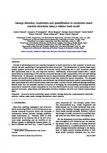
To demonstrate the performance of the proposed estimator we present several simulated experiments, all with a fiveomnidirectional-element uniform circular array. In the first experiment we compare the proposed estimator with other existing estimators in the case of white noise. The simulated scenario consisted of two equipower coherent Gaussian sources with 10-dB SNR's located at 100" and 120". The phase difference between the signals at the array center was 90". The array diameter was 0.6X, leading to a 3-dB

beamwidth of 26". A set of 100 Monte Carlo runs was carried out for each value of the number of snapshots, m, with the DOA's estimated in each run and the rms DOA error (averaged over the two sources) computed from the whole set. The results obtained by using the GLS, the weighted subspace fitting(WSF) [22],the deterministic ML (DML) [23], and the ML estimators, along with the CRB (derived in [12]) are displayed in Fig. 1. Clearly, the difference in the performance of these estimators is marginal. In the second experiment we demonstrate the performance for unequal noise power levels at the various sensors. The noise covariance was 22 = u2 . d i a g ( l , 2 , 4 , 2 ,l), where cr2 was chosen so that the SNR measured at the first sensor is 10 dB. The GLS estimator, using the noise model E = diag(a1. . . a s ) , was compared with the WSF, the ML, and the DML estimators all using a (incorrect) spatially whitenoise model. The results are shown in Fig. 2 and demonstrate ~the. advantage in using the GLS estimator in this case. To demonstrate the performance of the detection criterion we applied it to the first two experiments. The results are presented in Fig. 3. Clearly, the probability of correct detection approaches 1 as the number of available snapshots grows. To demonstrate the advantage in exploiting the fact that the sources are uncorrelated we show in Fig. 4 the CRB for four equipower uncorrelated sources located at loo", 120°, 140°, and 160". The noise is spatially and temporally white, and the number of snapshots is m = 256. The dashed line represents the CRB for the first source DOA error in case the prior knowledge about the lack of correlation is exploited, whereas the solid line represents the CRB in case this prior knowledge is not exploited. Notice that the performance difference is more conspicous at low SNR. VIII. CONCLUDING REMARKS We have presented a new method for detection and highresolution direction-finding in colored noise and in case the

WAX et ul.: DETECTION & LOCALIZATION IN COLORED NOISE

zal

1739

4-

L

cn (U F3.5-

0 L a,

3-

0)

E a

x

2.5

-

2-

- -1 0

(-100

1

200

400

300

500

600

number of samples

Fig. 2. Same scenario as in the previous figure except that here the spatial noise is nonwhite, with C = diag(1,Z. 4; 2 ; 1). -~

I: ' s -

~-

0 c ._

I

p

90-

d c 0

2?

..-.8

85-

0 . > e

-

E

2 80-

e L1

75 -

I

70'

signals are known to be uncorrelated. The DOA estimates derived are asymptotically efficient and have moderate computational complexity. The detection criterion is consistent. We have also pointed out that in case the signals are known to be uncorrelated it may be possible to localize them even if their number exceeds the number of sensors. A demonstration of this capability, as well as further discussion of the achievable performance, can be found in [ 121. APPENDIXA CONSISTENCY AND EFFICIENCY In this appendix we investigate the asymptotical behavior of the GLS estimator as the number of snapshots grows to infinity. We prove that the estimator is both consistent and asymptotically efficient.

A.I. Consistency

of

the GLS Estimates -1/2RR-lj2

The cost function !(4) = m/2111 - R ;1 in (12), whose minimizing value is the GLS estimator, is conA

tinuous and nonnegative. Therefore, to establish consistency it is sufficient to prove the following claims: 1) !(do) = 0; a s . m t cx, and 2) !(4) > 0 ; 4 # 4o a s . m + 00, where do denotes the true value of the parameters vector. Clairn 1) is clearly valid since R = R(4,) a.s. ni + CO, thus nullifying e( d o ) asymptotically. Claim 2) clearly holds due to the imiqueness assumption A3) that ensures that R ( 4 ) # R(q5,) for 4 # 40, implying that !(4) is asymptotically positive for 4 # 40.

A.2. E$ciency of the GLS Estimates We prove the efficiency of the GLS estimator by showing that asymptotically, as m -+ CO, it yields exactly the same estimation errors as the MLE which is known to be asymptotically efficient. The approach follows [ 11. To this end, let the operator vec(Z), acting on an m x rL matrix 2. output a vector of order mn 1 formed from the elements of z by concatenating its columns, i.e., if 2 denotes the zth column of 2 , then:

IEEE TRANSACTIONS ON SIGNAL PROCESSING, VOL. 44, NO. 7, JULY 1996

1740

L

def [ ( ZI ) ~(2 , 2 ) T , . .. ,(2 Also, let Z @ Y denote the Kronecker product of any two m x n , T x s matrices Z , Y , respectively, defined as the following mr x n s matrix: vec(2)

Z,lY

' . . Z,,Y

Using this notation it can be readily proved, see [6], that the following identity holds:

Now, let parameters:

4

denote a vector composed of all the real free

4

(eT,vet* ( P I ,

where k(4)= k-1'2R($)k-''2.The derivative of L G L ~ with respect to $%,the i-th component of 4, is given by

84%

- m &I

- R)]

and the derivative of a vector y E R m X 1with respect to a vector x E Rnx is defined by

dX

Similarly, the derivative of L M Lwith respect to

"'

4%is given

~~,

-1 L - -2 L aLrv'L(4)= m[tr(R R ) - tr(R R)] x

84%

H

= -m

(r)k)] dvec(R)

~ e c [ k - ~-( I

(A-7)

where we used

Using (A-l), this can also be written as

(A-8)

= -m t r [ R ( I - &)I = - m vecH(k) v e c ( 1 -

where the derivative of a scalar y with respect to a vector x E RnX' is defined by

(A-2)

where p is a real matrix formed from the free real parameters of the Hermitian matrix P in the following way: the elements on or above the diagonal of P are replaced by their real parts, while the elements below the diagonal are replaced by their imaginary parts. In case the signals are known to be uncorrelated, vec(P) is replaced by diag(P) in the above definition. Let $o denote the true value of 4. The GLS and the ML estimators are the values $GLS, &L minimizing, respectively, the following functions:

dLGLS(4)

where we have used the notation & def d k l d d , , and the identity t r ( A H B )= v e c H ( A ) _vec(B),and for notational convenience used the shorthand R for fi(q5). Thus

A)

(A-5)

Notice that since asymptotically k(4,) = I , and since the Kronecker product of any two identity matrices results in

WAX et al.: DETECTION & LOCALIZATION IN COLORED NOISE

1741

an identity matrix, so that [I @ fiP2(d0)]becomes asymp- v def (4, T ) , and rewrite the MDL criteria (31) and (33) as totically an identity matrix, it follows from (A-6) and (A-8) fi = argmin [MDL(v)] that the first derivatives d L ~ ~ ( $ ) / and d d i 3 L ~ ~ ~ ( d )are /dd v4I asymptotically identical at 4 = 4,. Assuming that U( 0) is twice continuously differentiable in MDL(v) e f m [ ( R c ( I $ ( v ) ) , Rkc, )logm (E-1) 2 m the neighborhood of $, it also follows that the matrices of second derivatives of L G L and ~ L M Lare continuous and both where $h(r’) def (0, P , a}represents all the parameters, with the have identical at 4 = $0 given by superscript noting that the size of $ is v-diependent, $(”I represents the GLS estimate, 1denotes the set of integer-pairs {v} for which v and d(,) can be uniquely determined, (., .) is the distance measure defined in (ll), and IC, denotes the total number of free parameters which is given by (32). Le1 q, denote the true number of signals and let r0 denote dzf the true noise model order, and define vo - (qo,T,) where where J ( 4 0 ) is given by we assume that v, E T. Also, let q5(’o) denote the true parameters. Now, to establish consistency we must pro\ e that asymptotically, with MDL(v) - MDL(v,) > 0 a.s. for v # v , , v E T (B-2)

+

def

F(q5) = plim lnim

d vec(R) -,

34

(A-11)

Notice that mJ($,) is in fact the Fisher Information Matrix (FIM). Now, expanding the first derivative expressions using the fact that at $GLS, $ML these derivatives are zero, we get

-I

To this enid we distinguish between two cases. 1) 0 5 q < qo or 1 5 T < T,: From (B-1) we get 1 m

-{MDL,(Y)

-

MDL(v,)}

= [{R(I$(”)),k) - (R($(l’o)),fi)] +

(B-3) where we asymptotically have R = R,, where R, denotes def the true covariance: R, = R($h(”.)). Now, asymptotically, R( # R,. since otherwise the uniqueness requirement (7) is viollated. Consequently,

8‘”))

( ~ ( $ ( , ) >) ,oka.s. )

3

where denotes a midpoint on the line segment joining the true value and the estimated value. Using and assuming that J ( $ , ) is full rank, we asymptotically get -

do = $GLs

-

4,

while (R($(”.)),k) = 0 a s . since $(”o) is a conzistent estimate and, therefore, asymptotically, R(d(”0))= k. = R, a.s. Consequently, the first term in (B-3) is a positive constant while the second term vanishes asymptotically, thus establishing (B-2). 2 ) v # v, and q 2 q, and T 2 T,: From (B-1) we get

MDL(Y) - MDL(v,)

= J - ~ ( ~ , ) F ~vec(1( $ ~ , R). ) (A-14)

03-4) Thus the asymptotic errors of the ML and the: GLS estimators are identical. APPENDIXB CONSISTENCY OF THE DETECTION CRITERION

To evaluate the asymptotic value of the first term we follow [27] and use the following result proved in [7, p. 1451. Lemma I : Suppose { e L i, 2 I} is a stationary real cp-mixing sequeince with E(e,) = 0,E(le,I2)< 30, and cp is decreasing with cp’/’((j) < CO. Then

”El

In this appendix we prove that our MDL based detection

criterion for estimating the number of signals is consistent. The proof applies even if the underlying distribution is not necessarily Gaussian. We deal with the more general case where both the noise model order T and the riiumber of signals q are unknown. To this end, we define the pair of integers

m

ei

lim sup m i m

where

i=l

(2m62log log m62)1/’

a2 ‘gfE(e:) + 2 E E l

E(elel+,)

= 1 as.

# 0.

I142

IEEE TRANSACTlONS ON SIGNAL PROCESSING, VOL. 44, NO. I , JULY 1996

Specifically, we apply this lemma to the elements of the error matrix [ z c ( t 2 ) z F ( t-7R,], ) and get

2 ) Case o f E = a21: For the case of spatially white noise, G and g are the following scalars obtained by substituting C1 = I (and consequently, 21 = k-’) into (22): G = tr(kP2) - t r ( PA(@ k P 1 ) ” g = t r ( P i ( e ) k - l ) , and the GLS

(B-5)

estimator (23) can be written as Also, by (A-14) and (B-5) we have ($,I - 4 (’)) = O ( d w ) a.s. and therefore, assuming that .(e) is continuous, we have from (6) that

R ( J ( ” )-)R, = 0

a.s. \

(B-6)

/

Now, expanding ( Y ,2 ) as a Taylor Power series around Y = R,,Z = R,, using the facts that (R,.R,) = 0;and that its first partial derivatives are zero (see [6]):

tr2 ( P ~ ( ~ ) K ~

8 = arg max e

. t r ( K 2 )- t r ( P - K A(@

(C-2)

’ ) 2

C.2. Uncorrelated Signals

To simplify the computation of e(8), in (27), we first partition the matrix G into the following blocks:

u w L

where using (26), we have we get that asymptotically ( Y ,2 ) can be approximated as a quadratic function of the elements of (Y - R,) and ( 2- R,). Therefore, by (B-5) and (B-6), we asymptotically get

m ( ~ ( $ ( ” ) ) ,=k O(1oglogm) t)

as.

This implies that the first term on the right-hand side of (B4) is asymptotically negligible when compared to the second term which is positive since k , > k,, , thus establishing (B-2). The so-called “penalty-term’’ used in the MDL criterion is kl,/210gm. Notice, however, that in fact we proved the consistency of the MDL criterion for any penalty term h,, strictly increasing with q and r , that obeys

v,j

u i j = ~ u y e ~ ) u ( e j ) ~ 2 ;= t r ( 2 & )

wtj

uH(s,)2ju(e,).

(C-3)

1

Now, using the following easily verified matrix inversion identity, valid for any full-rank symmetric matrix: [ZT

-[ -

r1-l Q

-V-lWTQ

-QWV-l V-l + V - l W T Q W V - l

I

where Q dLf (U - WV-’WT)-’, we can rewrite (27), omitting non-&dependent terms, as m t(0) = --(U - WV-lv)T[U - W v - l W y ( U - W v - l v ) lim k , / l o g l o g m i o o and m-m lim h,/m--tO. m i m 2 (C-4) Notice also that in fact we proved the consistency for any distance measure ( Y ,2 ) that is approximately quadratic near where U and v are two subvectors of g! such that gT = Y = 2.Also, the proof holds for any estimator whose (ur.vT).whose entries are given by ut = l\u(0,)ii2and asymptotic errors are o ( R - R). U, = t r ( 2 , ) . 1 ) Case of .E = diag(al. a2!. . , a p ) : For the special case APPENDIXC of an unknown diagonal E, a further simplification of the GLS FOR SOME SPECIAL CASES expressions for some of the terms in (C-4) is possible. Indeed, In this appendix, we give GLS expressions for the special repeating steps similar to those described in Appendix C.1-l), cases where E is either diagonal or a scaled identity matrix. we get (Q, = l(k-’),j12,(W)zj = I(AH(0)k-1),j12,v = In addition, we give a computationally simpler expression for diag(R-’). !(e) in (27). 2) Case o f E = (r21:For the case of uncorrelated signals in spatially white noise, we substitute r = 1 and 2 1 = k-’ C.1. Arbitrarily-Correlated Signals -2 -1 into (C-3), and get V = tr(R ) , U = tr(R ) , U = W = 1 ) Case of .E = diag(al,a2,...,oP): Using Zi = I,,,we -112 diag(AH(B)k-’A(o)). Substituting these expressions into (Chave ki = T;T?, where T ; denotes the ith column of R , 4), dropping non-&dependent terms, we get and consequently, by substituting this into (22),we get G,j = Ir?rjl2 - IrFPA(eIrj12and gL = rHP4 A(@r i , so that the 8 = min 0 { - ~ T[ tur - 1 ( K 2 ) ~ u ~ ] - 1 u } following expressions are used in the cost function (23): Now, using the matrix inversion lemma, we finally get A

\ ,

def

where diag(2) denotes a column-vector containing the diagonal elements of a square matrix 2.

where a(e) = UTU-’U, where 21 = diadAH(e)k-’A(e)) and ( U ) t j = /(AH(0)k-1A(O))LJ12.

WAX et ul.: DETECTION & LOCALIZATION IN COLORED NOISE

ACKNOWLEDGMENT The authors are grateful to one of the reviewers for bringing [ 131 to our attention. REFERENCES T. W. Anderson, “Linear latent variable models and covariance structures,” in J . Econometrics, vol. 41, pp. 91-119, 1989. l signals in J. F. Bohme, “Estimation of spectral parameters c ~correlated wavefields,” Signal Processing, vol. 11, pp. 329-337, 1986. J. F. Bohme and D. Kraus, “On least squares methods for direction of arrival estimation in the presence of unknown mise fields,” in Proc. IEEE Int. Conf on Acoust& Speech, and Signal Processing (ICASSP), New York, Apr. 1988, pp. 2833-2836. D. H. Brandwood, “A complex gradient operator and its application in adaptive array theory,” Proc. Inst. Elect. Eng. -pzrt H, on Microwaves, Optics, and Antennas, vol. 130, pp. 11-16, Feb. 1983. M. W. Browne. Covariance Struclures. Cambridge, U.K.: Cambridge Univ. Press, 1982, pp. 72-141. A. Graham. Kronecker Products and Matrix Cu1ch’lu.swith Applications. Chichester, UK: Ellis Horwood, 1981. P. Hall and C. C. Heyde. Martingale Limit Theory and its Application. New York: Academic, 1980. S. Haykin, Ed., Advances in Spectrum Analysis wid Array Processing, vol, 2. Englewood Cliffs NJ: Prentice Hall, 199 I . A. G. Jaffer, “Maximum likelihood direction fi,nding of stochastic sources: A separable solution,” in Proc. IEEE Int. Con$ on Acoustics, Speech, and Signal Processing (ICASSP), New York, Apr. 1988, pp. 2893-2896. D. H. Johnson and D. E. Dudgcon. Array Signa/ Processing. Englewood Cliffs NJ: Prentice Hall, 1991. J. Sheinvald and M. Wax, “Detection and localization of multiple signals using submays data,” in S. Haykin, Ed., Advances in Spectrum Analysis and Array Processing, Vol. 3. Englewood Cliffs, NJ: Prentice Hall, 1995, ch. 7, pp. 324-351. J. Sheinvald, M. Wax, and A. J. Weiss, “On the cramer-rao bound for localization of multiple signals,’’ IEEE Trans. Signal Processing, submitted for publication. D. Kraus and J. F. Bohme, “Asymptotic and empirical results on approximate maximum likelihood and least squares estimates for sensor array processing,” in Proc. IEEE Int. Con$ o.u Acoustics, Speech, and Signal Processing (ICASSPJ, Albuquerque, NM, Apr. 1990, pp. 2795-2798. J . P. LeCadre. Parametric methods for spatial signal processing in the presence of unknown colored noise fields. IEEE Trans. Acoust., Speech, Signal Processing, vol. 37, pp. 965-983, 1989. V. Nagesha and S. Kay, “Maximum likelihood estimation for array processing in colored noise,” in Pvoc. IEEE Int. Conf: on Acoustics, Speech, and Signal Processing (ICASSPJ Minneapolis, MN, Apr. 1993, pp. 4240-4243. A. Paulraj and T. Kailath, “Eignstructure methods for direction of arrival estimalion in the presence of unknown noise fields,” IEEE Trans. Acousl., Speech, Signal Processing, vol. ASSP-36, pp. 13-20, Jan. 1986. S. U. Pillai, Array Signal process in^. New York: Springer-Verlag, 1989. J. P. Reilly arid K. M. Wong, “Estimation of the directions of arrival of signals in unknown correlated noise-Part 11: Asymptotic behavior and performance of the map approach,” IEEE Trans. Signal Processing, vol. 40, pp. 2018--2028, Aug. 1992. J. Rissanen, “Modeling by shortest data description,” Autnmutica, vol. 14, pp. 465-471, 1978. P. Stoica, B. Ottersten, and M. Viberg, “An instrumental variable approach to array processing in spatially correlated noise fields,” in Proc. IEEE Int. Cor$ on Acoustics, Speech, and Signal Processing (ICASSPJ,, San Francisco, CA, Mar. 1992. A. H. Tewfik, “Direction finding in the presence of colored noise by candidate identification,” IEEE Trans. Signal Processing, vol. 39, pp. 1933-1942, Sept. 1991. M. Viberg, ‘Subspace fitting concepts in sensor arra:y processing,” Ph.D. dissertation, Ldnkopig Univ., 1989. M. Wax, Detection and eslimation of superimplosed signals. Ph.D. dissertation, Stanford Univ., Stanford, CA, 1985. -, “Detection and localization of multiple sfsurces in noise with unknown covariance,” IEEE Trans. Signcil Processing, vol. 43, July 1995.

1743

[25] IC. M. Wong et al., “Estimation of the directions of arrival of signals in unknown correlated noise-Part I: The map approach and its implementation,” IEEE Trans. Signal Processing, vol. 40, pp. 200;’~-2017, Aug. 11992. 1261 L,. C. Zhao. P. R. Krishnaia. and Z. D. Bai. “On detection of the lumber of signals in prescnce of white noise,” J. Multivariate Anal., vol. 20, pp. 1-25, 1986. [27] I. Ziskind and M. Wax, “Maximum likelihood localization of multiple sourceii by alternating projections,” IEEE Trans. Acou,st., Speech, Signal Processing, vol. 10, pp. 1533--1536, 1988.

Mati Wax (S’81-M’85-SM’88-~’’94) recei ied the B.Sc. and M.Sc degrees from the Technion Haifa, Israel, in 1969 and 1975, respectively, and thi: Ph D degree from Stanford University, Stanford, CA, in 1985, all in electrical engineering From 1969 to 1973 he served as an Electronic Engineer in the Israeli Army In 1974 Ire was with A E L , Israel In 1975 he joined RAFAEL, where he 15 currently heading the Center for Signal Processing In 1984 he was a Visiting Scientist at IBM Almaden Research Center, San Jose, CA. His research interests are in array signal processing and statistical modeliiig. Dr ’Wax is the recipient of the 1985 Senior Paper Award of the IEEE TRANSACTIONS ON ACOUSTICS, SPEECH AND SIGNAL PROCESSING

Jacob Sheinvald received the B Sc. and M. Sc. degrees from the Technion, Haifa, Israel, in 1974 and 1985, both in electrical engineering. He is currently working toward the Ph D. degree in the Department of Electrical Engineerlng-Systenl~,Tel Aviv University. From 1974 to 1979 he Eerved as an e1e:tronic engineer in the Israeli Army. In 1979 he joined RAFAEL, where he has been involved in research and development of communication syster s, and senror array processing During 1088-1990 he was a visiting scientist at IBM Almaden Research Center, San Jose, CA, working in the areas of pattern recognition and image analysis. His research interests are in array s,ignal processing and statistical modeling

Anthony J. Weiss (S’84-M’85-SM’86) received the B.Sc degree from the Technion, Haifa, Israel, in 1973, and the M.Sc. and Ph D. degree from Tel Aviv University, Israel, in 1982 and 1985, respectively, all in electrical engineering. From 1973 to 1983 he was involved in research and development of numerous projects in the fields of communications, command anal control, and direction finding. In 1985 he joineal the Department of Electncal Engineering-Systems, Tel Aviv L niversity During the academic year 1986-1987 he was a Visiting Scientist with the Laboratory for Information and Decision Systems, Massachusetts Institute of Technology. During 1987-1988 he was with Saxpy Computer Corp , Sunnyvale, CA, and during 1991-1992 he was with Signal Processing Technology, Palo Alto, CA. His research activities are Delection and Estimation Theory, Signal Processing, and Sensor Array Processing, with applications to radar and sonar Prof. Weis5 held a Rothschild Foundation Fellowship from 1986 tc 1987 and a Yigaal Alon Fellowship from 1985 to 1988 He was a recipient of the IEEE TRANSACTIONS ON ACOUSTKS, SPEECH, AND SIGNAL PROCESSING Socxty’s 1983 Senior Award for a paper excerpted from his Master thesis. In 15191 he received an award for his research contributions from the industry in Israel. During 1994- 1995 he has been the chairman of the IEEE Signal Processing chapter in Isr,ael Currently he serves as the chairman of IEEE Israel Stction.