Detection and Recovery From Pollution Attacks in Coding Based

1

Detection and Recovery From Pollution Attacks in Coding Based Distributed Storage Schemes Levente Butty´an, L´aszl´o Czap, Istv´an Vajda

N coding based distributed storage systems, data is stored in encoded packets in a distributed fashion, such that each encoded packet is computed by combining multiple data packets, according to the idea of linear network coding [1], [2]. In order to retrieve the original data, a sufficient number of encoded packets must be collected and decoded together. Such coding based distributed storage systems have important emerging applications, e.g. in peer-to-peer systems and in wireless sensor networks (WSNs). We consider multiple, distributed sources that generate data that must be stored efficiently in multiple storage nodes, each having constrained communication, computation, and storage capabilities. Storing encoded data, instead of raw data, can help to increase the efficiency of the system. In [3], [4], for instance, the following scheme is proposed: There are k source nodes, each producing a single data packet of interest (per time epoch), and there are n storage nodes that are used as a distributed memory for the k data packets. Each storage node can store a single data packet. Instead of storing raw data packets, each storage node stores a linear combination of a subset of them. The random coding techniques (distributed erasure codes, fountain codes) introduced in [4], [5], [6] ensure that, for appropriately selected parameters, a collector node can reconstruct all the k data packets with high probability by downloading the encoded packets from any k storage nodes and solving a system of linear equations (s.l.e). Thus, the collector node can retrieve the interested data from k nearby nodes, which results in decreased delay in data reconstruction and lower traffic load in the network.

While coding may increase the efficiency of distributed storage systems in a benign environment, it also has a potential problem in hostile environments, where an adversary may attack the storage nodes. In particular, the problem that we are interested in this paper is the so called pollution attack [7], whereby the adversary modifies some of the stored encoded data, which results in erroneous decoding of a large part of the original data upon retrieval. Note that these coding schemes mix (typically, linearly combine) blocks of the original data, therefore, a single corrupted encoded block can affect the decoding of multiple data blocks. This amplification effect of the pollution attack is particularly annoying and undesirable. Our main contribution in this paper is a novel information theoretic approach to counteract pollution attacks in coding based distributed storage systems1 . Compared to other approaches in the same vein, we do not add redundancy to the data packets, but rather, we take advantage of the inherent redundancy provided by the coding scheme itself. This redundancy comes from the fact that the content of each storage node corresponds to the same data block vector. To the best of our knowledge, our proposal is the first error detection/correction method that does not require any new functionality at the source nodes or at the storage nodes. The price of this property is only a slightly increased communication overhead for the attack detection. On the other hand, the attack recovery requires more computational effort from the collector. While the scheme we describe is general, we illustrate its benefits in the context of WSNs where requirements on resource consumption are the most demanding. The principles of our algorithms can be extended also for network coding based P2P file distribution systems, because the algorithms and analysis do not exploit any specialties of WSNs that would hinder their application in other storage systems. We propose algorithms for pollution attack detection and also for recovery from such attacks. In order to measure the performance of our algorithms, we calculate the probability of success together with the complexity of the algorithms. Two complexity measures are considered: the computational complexity, measured in the number of s.l.e.’s that need to be solved, and the communication complexity, measured in the number of encoded packets that need to be downloaded when data is retrieved from the distributed storage system. We showed the optimal communication and computational complexity of the proposed attack detection algorithm in the

L. Butty´an, L. Czap and I. Vajda are with the Laboratory of Cryptography and Systems Security, Budapest University of Technology and Economics, 2. Magyar tud´osok krt., H-1117 Budapest, Hungary

1 The first version of this work was presented in [8]. Here we apply a stronger adversary model and develop further algorithms for the recovery problem.

Abstract—We address the problem of pollution attacks in coding based distributed storage systems. In a pollution attack, the adversary maliciously alters some of the stored encoded packets, which results in the incorrect decoding of a large part of the original data upon retrieval. We propose algorithms to detect and recover from such attacks. In contrast to existing approaches to solve this problem, our approach is not based on adding cryptographic checksums or signatures to the encoded packets, and it does not introduce any additional redundancy to the system. The results of our analysis show that our proposed algorithms are suitable for practical systems, especially in wireless sensor networks. Index Terms—Network level security and protection, sensor networks, distributed data storage, network coding, pollution attack, integrity protection

I. I NTRODUCTION

I

2

X1

X2

Xk ...

Zj

1

k source nodes

n 1

G ...

G

... k

...

Z2

x

Zn Zj = (Gj, Yj) = (Gj, XGj)

1

k

Gj

G1 G2

Gn

1

n 1

1 X

...

Z1

n storage nodes

...

...

...

Y m

m

collector node(s)

Fig. 1.

System model.

X1 X2

Xk

Y1 Y2

Yj

Yn

Fig. 2. Illustration of the system of linear equations representing the entire distributed storage system.

applied system model. We investigate the attack recovery problem as well. We show an algorithm with very low computational complexity. We also propose a recovery algorithm with optimal communication complexity, which has also feasible computational complexity for small to medium size practical systems. For larger systems, we propose a recovery algorithm that makes a trade-off between the two complexity measures. We also introduce an extension of the recovery algorithms to reduce the false negative error probability in the case of a strong adversary. The remainder of the paper is organized as follows: In Section II, we introduce the system model and the adversary model. In Section III, we describe our proposed attack detection algorithm, together with the analysis of its error probability and complexity. In Section IV, specific recovery algorithms are proposed and analyzed. Section V gives the extension of the recovery algorithms. In Section VI, some related works are discussed, and finally, in Section VII, we draw some conclusions. The appendix contains some additional computations and results. II. M ODEL A. System model The general model of the distributed storage systems that we consider in this paper is taken from [4] and it is illustrated in Figure 1. The system consists of k source nodes, n storage nodes, and one or more collector nodes. Note that these are roles, and therefore, the sets of source nodes, storage nodes, and collector nodes may overlap. Only the collector node is assumed to be a powerful computer (base station), while source and storage nodes may be low capacity devices. Each source node i generates a data block Xi , and transfers it to some randomly selected subset of the storage nodes. Each storage node j computes a random linear combination of all the data blocks that it receives; the result is a single code block Yj . Formally, we can write that Yj = XGj , where X = (X1 , X2 , . . . , Xk ) is the row vector of all the data blocks, and Gj = (g1j , g2j , . . . , gkj )T is a column vector, the non-zero elements of which are the random coefficients used in the linear combination. Here, gij ∈ GF (q) for all i = 1, 2, . . . , k and j = 1, 2, . . . , n, and for some q. Each storage node j stores the pair Zj = (Gj , Yj ), which represents the equation Yj = XGj . The entire system is represented by the system of linear equations (s.l.e.) Y = XG, where Y = (Y1 , Y2 , . . . , Yn ) is the row vector of all code blocks, and G = (G1 , G2 , . . . , Gn ) is a

k×n matrix that contains the coefficient vectors in its columns. Matrix G is also called generator matrix. For appropriately selected values of k and q, any k × k submatrix of G is non-singular with high probability. According to Theorems 1 and 2 in [4], the probability of non-singularity is at least (1 − kq )c2 (k), where c2 (k) → 1, if k → ∞. Larger values of q increase the probability of successful decoding, but makes the overhead of storage higher. [4] also shows that storage nodes required to store O(ln k) coefficients. E.g. if k = 100 and q = 220 , the probability of singularity is ≈ 10−4 , while the average overhead of a storage node is 92 bits. Therefore, the collector node can reconstruct all the data blocks with high probability by downloading the equations from any k storage nodes and solving the obtained s.l.e. for X. In the rest of the paper, we assume that this property of G holds. In fact, each data block Xi can itself be a column vector of m symbols (x1i , x2i , . . . , xmi )T , where xℓi ∈ GF (q) for all i = 1, 2, . . . , k and ℓ = 1, 2, . . . , m. In that case, each code block Yj is also a column vector (y1j , y2j , . . . , ymj )T of m symbols in GF (q). The linear combination Yj = XGj is computed in a symbol-by-symbol manner, meaning that yℓj = Pk i=1 xℓi gij for all j = 1, 2, . . . , n and ℓ = 1, 2, . . . m. Thus, one can think of X and Y in the s.l.e. Y = XG as matrices of size m × k and m × n, respectively. This view is illustrated in Figure 2. B. Adversary model We assume that the adversary has access to t storage nodes, and she can observe and modify the equations stored by them. This means that if the adversary has access to storage node j, then she can modify both Gj and Yj stored by node j. Let G∗ = G + ∆G and Y ∗ = Y + ∆Y be the modified generator matrix and the modified code block vector after an attack, where the modifications made by the adversary are contained in matrix ∆G and vector ∆Y . We further allow the adversary to compromise the communication links of the t storage nodes. It gives more possibility to the adversary, but does not extend the possible effect of the attack. For simplicity, we refer to nodes that store modified data as compromised nodes, and not distinguish them upon the way of modification. Note that the adversary has no access to the source nodes, rather she aims at compromising the output of the storage system. The rationale behind this assumption is that storage nodes are exposed to attacks for an extended period of time, whereas

3

the source nodes must be attacked during the limited time period of data generation. Data distribution from the source nodes to the storage nodes typically takes place on a wireless channel, that is exposed to various attacks. Accordingly, our applied model of adversary is realistic in most cases. Recall that when reconstructing the data blocks, the collector node chooses the k storage nodes, from which it downloads the k linear equations, randomly. Therefore, the adversary has no information on which storage nodes will be chosen when she performs the attack. At the same time, the collector node does not know which storage nodes are compromised. In the sequel, we will assume without loss of generality that the adversary randomly chooses the t storage nodes to be compromised, and the collector node downloads the equations of the first k storage nodes, where the order of the storage nodes is defined randomly by the collector node. Thus, the set of equations downloaded by the collector node is ∗ ∗ Z1..k = (G∗1..k , Y1..k ), where G∗1..k = (G∗1 , G∗2 , . . . , G∗k ) and ∗ ∗ ∗ Y1..k = (Y1 , Y2 , . . . , Yk∗ ). Let us now investigate the effect of an attack. The collector ∗ node solves the s.l.e. Y1..k = XG∗1..k for X, and obtains the ∗ (G∗1..k )−1 . Let us suppose for the moment result X ∗ = Y1..k that the adversary modifies only the code blocks, meaning that ∗ G∗ = G. In this case, X ∗ = Y1..k (G1..k )−1 . The modification induced by the attack in the decoded data blocks can be computed as follows: ∆X = X ∗ − X ∗ = Y1..k (G1..k )−1 − X = (Y1..k + ∆Y1..k )(G1..k )−1 − X = ∆Y1..k (G1..k )−1 where in the last step we used that Y1..k (G1..k )−1 = X. This means that (a) if a given row of ∆Y1..k contains only zeros, then the corresponding row of ∆X will contain only zeros too, and (b) a non-zero element in a given row of ∆Y1..k will affect the entire corresponding row in ∆X. Thus, a modification made by the adversary in a given row in any of the first k code blocks will, in general, affect all decoded data blocks, but the effect will be limited to the corresponding row. This is illustrated on the left hand side of Figure 3. Now, let us suppose that the adversary modifies only the coefficient vectors, meaning that Y ∗ = Y . In this case, X ∗ = Y1..k (G∗1..k )−1 . If at least one of the first k coefficient vectors has been modified by the adversary, then G∗1..k 6= G1..k , and thus, (G∗1..k )−1 can be completely different from (G1..k )−1 . Therefore, in general, such a modification affects all decoded data blocks in every row. This is illustrated on the right hand side of Figure 3. If the adversary modifies both the coefficient vectors and the code blocks, then these effects are combined. In the general case, the modification induced by the attack on the decoded data blocks can be derived as follows: X + ∆X = (Y1..k + ∆Y1..k )(G∗1..k )−1 (X + ∆X)G∗1..k = Y1..k + ∆Y1..k X∆G1..k + ∆XG∗1..k = ∆Y1..k ∆X = (∆Y1..k − X∆G1..k )(G∗1..k )−1

where in the second step we used that G∗1..k = G1..k +∆G1..k and XG1..k = Y1..k . The above formulas imply the following observation. If ∆Y1...k is controlled by the adversary, meaning that all downloaded equations are from compromised nodes, the value of ∆X can be chosen by the adversary. The adversary can reconstruct X from the contents of the nodes, so she is able to enforce arbitrary X ∗ = X + ∆X solution by loading Yi∗ = Xi∗ Gi as the modified content of the i-th compromised storage node. As a result, the adversary can not only destroy the original data block vectors, but she can also enforce a particular value. This scenario may occur, if t ≥ k. Actually, these observations illustrate the amplification effect of the pollution attack: a small amount of modifications in the stored coded information can result in a large amount of modifications in the decoded data. In the worst case all data blocks are entirely destroyed. This is highly non-desirable, and requires the development of some countermeasures. Below, we address this problem by proposing mechanisms to detect and recover from such attacks. III. ATTACK DETECTION A. Principle The basic idea of our attack detection mechanism is the following: In most cases, the adversary cannot enforce a ∗ particular solution X ∗ = Y1..k (G∗1..k )−1 , because it is unlikely that she compromises all the first k equations (the probability (t) of this event is nk ≈ (t/n)k ). In most of the cases, X ∗ can (k) be treated as a random vector, except if all the first k equations are intact, in which case X ∗ = X will hold. As we will see from the alysis, if X ∗ 6= X, X ∗ takes its values randomly form a set of size at least q. Now, suppose that we have an additional intact equation: Yk+1 = XGk+1 (i.e., the collector downloaded Zk+1 = (Gk+1 , Yk+1 )). If X ∗ is random or it is chosen by the adversary, then it will not satisfy the additional intact equation with high probability, while it will satisfy it with probability 1 if X ∗ = X. Thus, we can detect if the decoded data block vector X ∗ is polluted with the help of an additional intact equation. In the rest of this section, we develop an attack detection algorithm based on the principle described above, and we analyze it in a more rigorous way. B. Algorithm The proposed attack detection algorithm works in the following way: The collector downloads the first k equations ∗ ∗ Z1..k and computes X ∗ = Y1..k (G∗1..k )−1 . Then, the collector ∗ ∗ downloads the next equation Zk+1 . If Yk+1 = X ∗ G∗k+1 , then no attack is detected (and the collector accepts X ∗ as the ∗ 6= X ∗ G∗k+1 , an attack is correct solution). Otherwise, if Yk+1 signalled. C. Analysis In this subsection, we investigate the complexity of the attack detection algorithm, as well as its false negative and false positive error probabilities.

4

1

1

k 1 (G1..k)-1 k

x 1

k

1

1 xxxxxxxxxxxxxxxxxxxxxxxxxxx xxxxxxxxxxxxxxxxxxxxxxxxxxx xxxxxxxxxxxxxxxxxxxxxxxxxxx

m

Fig. 3.

1

1 xxxxx xxxxx xxxxx

Y*1..k

x 1

k X* m

Y1..k m

k

k

xxxxxxxxxxxxxx 1 xxxxxxxxxxxxxx xxxxxxxxxxxxxx xxxxxxxxxxxxxx xxxxxxxxxxxxxx xxxxxxxxxxxxxx xxxxxxxxxxxxxx xxxxxxxxxxxxxx xxxxxxxxxxxxxx k xxxxxxxxxxxxxx 1

(G*1..k)-1

k

xxxxxxxxxxxxxx 1 xxxxxxxxxxxxxx xxxxxxxxxxxxxx xxxxxxxxxxxxxx xxxxxxxxxxxxxx m xxxxxxxxxxxxxx

X*

Effects of the pollution attack on the decoded data blocks.

1) Complexity: We measure the communication complexity in the number of downloaded equations. This measure is a property of the algorithm independently of the network topology, however describes well the amount of communication required. The amount of traffic that loads the network in reality highly depends on the topology and routing. The computational complexity in the number of s.l.e.’s that the collector needs to solve. Again this is an abstract measure that describes the algorithms. The amount of required computation depends on the size of the system. We can expect that an s.l.e. can be solved in O(k 2.5 ) steps. For recovery we introduce an acceleration that makes this computation faster. For simplicity we do not consider the method of solving s.l.e.’s when describing the algorithms and complexity refers only the number of solved s.l.e.’s. The communication complexity of the proposed attack detection algorithm is hence k + 1, and its computational complexity is 1. According to Lemma 1, any attack detection algorithm that operates in the described system needs at least k + 1 equations to download, hence the attack detection is optimal in terms of communication complexity. Lemma 1: In the described system model, any attack detection algorithm uses at least k + 1 downloaded equations. Proof: When a node downloads k ′ equations, the obtained matrix G∗1...k′ determines a (k ′ , k) linear code for the data ∗ block vectors where Y1...k ′ is the coded block vector. An attacked encoded block can be seen as an erroneous block. Note, that the case when not only the coded block but the encoding vector is also modified, can be treated as if only the encoded block was modified, because each encoding vector is valid, thus it has a corresponding correct encoded block. It is known that the Hamming distance of any error detection code is at least 2. In our case, k ′ determines the Hamming distance of the code. If k ′ < k, the Hamming distance is 0, because the s.l.e. has many solutions, thus many data block vectors have the same encoded vector. When k ′ = k, the Hamming distance of the code is 1, because each encoded block is valid and has exactly one corresponding data block vector. This is sufficient for decoding, but not for error detection. It means, that attack detection is not possible with less than k + 1 equations. If k ′ = k + 1, the Hamming distance reaches 2, because the last coded block is determined by the first k blocks, thus error detection becomes possible. 2) Probability of a false negative decision: We distinguish two cases: either X ∗ can be taken as a random value, or it is controlled by the adversary. First, we assume that either out of

the first k downloaded equation at least one equation is intact, or the adversary modified the content of the storage nodes independently, thus X ∗ can be taken as a random value. Let us assume for the moment that the adversary does not modify the coefficient vectors, meaning that G∗ = G. As we saw earlier, in this case, the collector obtains the solution X ∗ = X + ∆Y1..k G−1 1..k = X + ∆X. If we further assume that the additional equation that we ∗ use for detection is intact, then we have Zk+1 = Zk+1 = (Gk+1 , Yk+1 ). In this case, the false negative error probability, denoted by Pfneg , can be computed as follows: Pfneg = Pr{Yk+1 = X ∗ Gk+1 |∆Y1..k 6= 0} = Pr{Yk+1 = (X + ∆X)Gk+1 |∆Y1..k 6= 0} = Pr{∆XGk+1 = 0|∆Y1..k 6= 0}

(1)

where in the last step we used that Yk+1 = XGk+1 . Recall from the left hand side of Figure 3 that if ∆Y1..k has a non-zero element in the i-th row (and G1..k is intact), then ∆X also has some non-zero elements in the i-th row. Otherwise, if the i-th row of ∆Y1..k contains only zeros, then the i-th row of ∆X contains only zeros too. We can write the i-th element of ∆XGk+1 as k X

∆xiℓ gℓ(k+1)

(2)

ℓ=1

By the argument above, (2) is a non-trivial linear combination of the elements of Gk+1 . However, the elements of Gk+1 are chosen randomly and due to the random order of downloads, these values are not known to the adversary in advance, therefore, the probability of (2) being 0 is equal to 1/q. If elements of ∆X are independent, Pfneg =

1 q t′

(3)

where t′ is the number of rows in ∆Y1..k that contain non-zero elements. When the modifications are dependent, Pfneg ≤ 1/q is still true. From this, it follows that X ∗ takes its value randomly from a set of size at least q. Clearly, in order to maximize the error probability (and hence minimize the success probability) of the detection, the adversary must make all modifications to the code blocks in a single row, or make the modifications of rows linearly dependent. Next, we keep the assumption that the adversary does not modify the coefficient vectors (hence G∗ = G), but we assume that the code block of the additional equation that we use for

5

∗ ∗ detection is attacked, meaning that Zk+1 = (Gk+1 , Yk+1 )= (Gk+1 , Yk+1 + ∆Yk+1 ). In this case, a simple derivation similar to the previous case can be used to arrive to the following result:

Pfneg = Pr{∆XGk+1 = ∆Yk+1 |∆Y1..k 6= 0}

(4)

Recall from the previous discussion that the i-th row of ∆X contains only zeros if the i-th row of ∆Y1..k contains only zeros. In this case, the i-th element of ∆XGk+1 must be a zero too. Thus, if the i-th element in ∆Yk+1 is not zero, then the above error probability is 0 (i.e., we can detect the attack even though the additional equation used for detection is not intact). On the other hand, if ∆Yk+1 contains zeros in every row where ∆Y1..k contains only zeros, then due to the randomness of Gk+1 , we get again that Pfneg ≤ 1/q. Finally, let us consider the general case when the adversary may modify both the coefficient vectors and the code blocks, hence ∆G 6= 0 and ∆Y 6= 0. This case has to be ∗ handled carefully, because X ∗ = Y1..k (G∗1..k )−1 might be not completely random. E.g. if ∆Y1..k = X∆G1..k then although ∆G1..k 6= 0 and ∆Y1..k 6= 0 can hold, ∆X = 0. Of course this modification can not be treated as an attack, because the modified equation is not polluted. This example is to point out that even if all elements of the coefficient vector and the encoded block are modified it may be equivalent to an intact equation with a single modified element. Thus, if we consider the highest possible dependency between modified elements, we get back to the previous case, and ∗ Pfneg = Pr{Yk+1 = X ∗ G∗k+1 |∆G1..k 6= 0} ≤

1 q

(5)

holds also for this case also. In the case of a random adversary, all values of X ∗ may be independently random, and hence this probability falls to 1/q m . The conclusion of this analysis is that when not all downloaded equations belong to the same X ∗ 6= X value, the maximum value of a false negative detection is Pfneg = 1/q. Hence, if q is chosen sufficiently large, then the probability of not detecting a pollution attack is negligible. Of course a larger value of q introduces larger overhead in communication and storage also. Note that if the code blocks contain standard error detection elements, such as a CRC checksum, then at least 2 rows must be changed presumably independently by the adversary in every attacked code block. Consequently, in that case, we have that Pfneg ≤ 1/q 2 . This observation allows to choose smaller fields and hence to make the computations over the Galois field faster. Recall from the system model that e.g. q = 220 is realistic, that indicates an error probability 2−40 . Now, we consider the case when all k + 1 downloaded equations are polluted and X ∗ is chosen by the adversary. In this case the attack detection algorithm does not signal an attack, because X ∗ satisfies the polluted testing equation also. This is clearly a false negative decision. The probability of ( t ) ≈ (t/n)k+1 . When t is not very large this case is ∆ = k+1 n ) (k+1 compared to n and k is large enough, this value is very small (e.g. when n = 100, k = 10, t = 20, ∆ ∼ 10−9 ). Hence,

we can estimate the upper bound of a false negative decision with: Pfneg < 1/q + ∆. Beside k, the value of ∆ depends on the number of compromised nodes. In most cases, it is reasonable to assume that n ≫ t, and so ∆ is close to 0. However, if we consider a strong adversary and large values of t, ∆ may become not negligible. In Section V we give a method to eliminate the effect of ∆. 3) Probability of a false positive decision: Let us close this section with the analysis of the probability of a false positive decision. For this, let us assume that the first k equations downloaded by the collector node are intact, meaning that ∗ Z1..k = Z1..k . Thus, the collector computes the correct ∗ solution X ∗ = Y1..k (G∗1..k )−1 = Y1..k (G1..k )−1 = X. If the additional equation downloaded for attack detection is also ∗ = Zk+1 ), then no attack is detected as intact (i.e., Zk+1 ∗ Yk+1 = Yk+1 = XGk+1 = X ∗ G∗k+1 . Thus, an attack may be signaled only in the case when the additional equation is not intact. From this, a good approximation of the probability of a false positive decision, denoted by Pfpos , is the following: Pfpos ≈ Pr{∆Zk+1 6= 0|∆Z1..k = 0}

(6)

Given that the first k equations are intact, the probability that the (k + 1)-st equation is also intact is
n−k−1 n−k−t t (7)
= n−k n−k t

where t is the number of randomly chosen storage nodes that are attacked by the adversary. From this, we get that

n−k−t t = (8) n−k n−k While Pfpos is not negligible, false positive decisions do not have serious effects. Indeed, when the attack detection algorithm signals an attack, the recovery procedures described in the next section are executed. These procedures try to recover the original data block vector, and as we will see, they succeed in a few steps when the number of attacked equations is small (which is the true by definition in case of a false positive decision of the attack detection algorithm). Pfpos = 1 −

IV. R ECOVERY

FROM ATTACK

Based on the same principle as the attack detection, we give recovery algorithms as well. These algorithms use the attack detection algorithm as a building block. The task of the recovery algorithm is to find a k + 1 size set of intact equations, given the attack detection algorithm. With less than k + 1 intact equations, successful recovery is theoretically impossible, because k intact equations are needed to obtain the correct data block vector and an additional intact equation is needed to verify the solution. The attack detection is assumed to always give correct result, because q can be chosen sufficiently large and ∆ is negligible. Later in Section V we investigate cases when this assumption is too strong, i.e. when the attacker is strong enough to compromise a large portion of the storage nodes.

6

TABLE I M AIN PROPERTIES OF THE PROPOSED RECOVERY ALGORITHMS

9

10

8

Communication complexity

Computational complexity

optimal optimal reasonable

high optimal medium

low high medium

Average computational complexity (log scale)

Algorithm 0 Algorithm 1 Algorithm 2

Success probability

10

n=100, k=10 n=500, k=50 n=600, k=50 n=1000, k=100

7

10

6

10

5

10

4

10

3

10

2

10

1

10

20

Fig. 5.

Fig. 4. Comparison of the three recovery algorithms - the left hand side group belongs to n = 100, the right hand side group belongs to n = 1000.

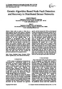
In other words, the attack detection algorithm gives for any k + 1 size set whether it contains some polluted equations or not. If an attack is signaled, we only know that there are some polluted equations in the set, but do not know how many and which
ones. Therefore, the system
can be modeled as n n−t Z = k+1 sets out of which z = k+1 are intact and we need to find one of the intact sets. In the following three subsections we propose three specific algorithms for the recovery problem. The first two of them have optimal success probability, meaning that if recovery is possible, they eventually succeed. Table I summarizes the main properties of our algorithms, while Fig. 4 illustrates the qualitative properties of the algorithms for two representative systems, a small and a large one, having (n, k, t) ∈ {(100, 10, 40), (1000, 100, 80)}2. This figure gives an overview of the algorithms, while we give the detailed analysis of each later. In computational complexity Algorithm 0 is near to the optimum, but has high communication complexity. On the contrary, Algorithm 1 has the theoretical optimum with respect to communication complexity, but has unfeasibly large computational load for a large system. Our third algorithm gives up the optimality of success probability to fit for large systems in complexity. A. Algorithm 0 1) Description: Let us choose randomly a k +1 size set out of the n equations of the system. Let S be the first k element in this set. Run the attack detection algorithm on set S with the remaining equation as the testing equation. If no attack is 2 Algorithm 2 has a further parameter τ max , we introduce later, we set τmax = 4 in the figure. Although the success probability of Algorithm 2 is not optimal, we will see later, that for these values this hardly makes sense.

40

60 80 100 Number of attacked equations (t)

120

140

160

Average computational complexity of Algorithm 0

signalled, S is clear. Otherwise, restart the algorithm with a different randomly chosen set. 2)
Computational complexity: The algorithm tests the Z =
n n−t sets until it fonds one of the z = intact sets. k+1 k+1 The expected value of the computational complexity of Algon )+1 (k+1 rithm 0 is hence Z+1 z+1 = (n−t)+1 . Fig. 5 shows the average k+1 computational complexity as the function of the number of attacked equations in the system for some selected values of n and k. The figure clearly indicates the exponential complexity, but also shows that in practice the range of usability is quite wide, for n = 100 nodes and k = 10, if 70% of the nodes are attacked, the complexity is still below 107 , and in a ten times larger system (n = 1000, k = 100), with the same complexity still more then 15% of the nodes can be attacked. Furthermore, there are reasons to assume that the exponential complexity can not be avoided in this system model. Our conjecture is as follows: Having n equations, fixed k value and an unknown number t of attacked equations in the system, if any algorithm provides optimal success probability, the lowest average computational complexity it may have is exponential in t. 3) Communication complexity: The following approximation is used to estimate the communication complexity of Algorithm 0. In each iteration the probability that a given equation is selected is k+1 n , as k+1 equations are selected randomly out of the n equations. This consideration holds if the same s.l.e. is allowed to be selected multiple times (if the selection of the iterations are independent). Our approximation is good for Algorithm 0, if Z ≪ Z+1 z+1 . This holds for the typical parameters in practice. Accordingly, the system is treated as n independent random variable having geometric distribution with parameter k+1 n . The jth equation is downloaded in the ith iteration, if the value of the jth variable equals i. From the geometric distribution it follows, that after the ith iteration of the algorithm, the expected number of downloaded equations is ω−1   i  X k+1 k+1 1− . n n n ω=1 The expected value of the communication complexity is the weighted average of these values with the probability that

7

Algorithm 0 stops in the ith iteration as weights. The success probability of Algorithm 0 can be estimated with Zz in each iteration, thus it succeeds in the ith iteration with probability
i−1 z 1 − Zz Z . Again, we model the iterations as independent selections of sets. As a result, the estimated communication complexity of Algorithm 0 is i−1   i  ∞ k+1 k+1 z i−1 X z X 1− . 1− n Z i=0 Z n n j=1 The complexity increases rapidly with the number of attacked equations. Fig. 4 already showed the high complexity of this algorithm. This is the main drawback of Algorithm 0, because in sensor networks it is important to minimize communication complexity. In the following we present Algorithm 1, that has optimal communication complexity. B. Algorithm 1 1) Principle: The following two recovery algorithms are both based on the same principle. When the collector node ∗ detects that the originally downloaded set S = Z1..k of equations is polluted, it can download more equations and use them to clean the polluted set S. The basic idea of cleaning is the following: Let us denote the set of equations downloaded for cleaning by C, and let e be an additional equation. We use the equations in C to replace a subset of size |C| of the equations in S. We denote the resulting new set of equations by S ′ . Then, we run our attack detection mechanism on S ′ with equation e used for testing. In other words, we solve the s.l.e. corresponding to S ′ and check if the solution satisfies equation e. If no attack is detected, then we accept the obtained solution as the correct data block vector. Otherwise, we take S again, replace another subset of size |C| of its equations, and run the attack detection again. We repeat these steps until either the cleaning succeeds or all possible subsets of size |C| of set S has been replaced. Note that if e is intact, C contains only intact equations, and the number of the attacked equations in S is not greater than |C|, then the above described procedure eventually succeeds, because we will eventually replace all the attacked equations in S by the intact equations in C. In case of failure, either e is attacked, or C contains an attacked equation, or the number of attacked equations in S is greater than |C|. In this case, we may download another set C ′ of equations such that |C ′ | > |C|, as well as another testing equation e′ , and try the cleaning of S again. In the rest of this section, we propose two specific recovery algorithms based on this principle. As we will see, the first algorithm is optimized for communication complexity, however, its computational complexity does not scale well with k. Nevertheless, it is still usable for many practical systems. The second algorithm that we propose has improved computational complexity, however, in general, it has a higher communication complexity than the first algorithm has, and it can recover only from attacks where the number of the compromised storage nodes is limited. We deliberately do not give more precise statements about the performance of our algorithms at this

point. We analyze them and describe the trade-off that they offer in more details below. 2) Description: The basic idea of our Algorithm 1 is to start the cleaning with a cleaning set C of size one (i.e., to assume first that there is only one attacked equation in set S), and then, if cleaning fails, to increase the size of C iteratively. In this way, sooner or later, we arrive to a cleaning set C that contains as many intact equations as the number of attacked equations in S. In each iteration, we select all possible subsets of the equations in C and replace with them all possible subsets of equations in S. Thus, eventually, we replace the attacked equations with the intact ones, and arrive to a clean set. Below, we first formalize the operation of the algorithm, then analyze its success probability and complexity. The pseudo-code of the algorithm is presented in Table II. Its operation is explained as follows: The algorithm first ∗ downloads Z1..k+1 (line 1) and runs the attack detection ∗ ∗ algorithm on Z1..k using Zk+1 as the testing equation (line 2). ∗ If no attack is detected, then Z1..k is clean and the algorithm stops (line 3). Otherwise, the algorithm starts the cleaning of ∗ S = Z1..k (lines 5–24). This is an iterative process, where in each iteration (lines 7-24), exactly one new equation is downloaded (line 8). The newly downloaded equation, denoted by e, becomes the testing equation used for attack detection in the current iteration (line 10). The rest of the equations downloaded so far, not counting the equations in S, constitute the cleaning set denoted by C (line 9). The algorithm takes every possible subset C ′ of C, such that |C ′ | = τ is not greater than k (lines 12–13), and uses the equations in C ′ to replace τ equations in S in all possible ways (lines 14– 16). After each replacement, the attack detection mechanism is executed on the resulting set S ′ of equations using e as the testing equation (line 17). If no attack is detected, then S ′ is clean and the algorithm stops (line 18). 3) Success probability: It is easy to see that the algorithm succeeds iff the number t′ of the attacked equations in S = ∗ Z1..k is smaller than the number of the intact equations in ∗ . On the one hand, if this condition the remaining set Zk+1..n ∗ holds, then we have at least t′ + 1 intact equations in Zk+1..n , and therefore, as we continue downloading more and more equations for cleaning, we eventually reach a state where the cleaning set C contains at least t′ intact equations and the last downloaded equation e used for attack detection is also intact. In this case, eventually, all the attacked equations in S will be replaced by intact equations from C, hence S will be cleaned. In addition, as e is intact, the attack detection mechanism will indicate no attack, and we can actually realize that S is cleaned. On the other hand, if t′ is not smaller than the number of ∗ the intact equations in Zk+1..n , then either the cleaning set C ′ contains fewer than t intact equations, and hence, S cannot be cleaned, or C contains exactly t′ intact equations and S can be cleaned, but we have no more intact equation for attack detection purposes, and therefore, we cannot realize that S is cleaned. Given that there are t attacked equations all together, and t′ ∗ of them are in Z1..k , we get that the number of intact equations

8

1 2 3 4

∗ download Z1..k+1 ∗ , Z∗ if attack detection(Z1..k k+1 ) = no attack ∗ return Z1..k endif

S

∗ 5 let S = Z1..k 6 let w = 1 7 while w < n − k ∗ 8 download Zk+w+1 ∗ 9 let C = Zk+1..k+w ∗ 10 let e = Zk+w+1 11 for τ = 0 to min(w, k) 12 for every possible selection s1 of τ elements out of w elements 13 let C ′ be the subset of equations determined by s1 in C 14 for every possible selection s2 of τ elements out of k elements 15 let S ′ = S 16 replace the equations determined by s2 in S ′ with the equations in C ′ 17 if attack detection(S ′ , e) = no attack 18 return S ′ 19 end if 20 end for 21 end for 22 end for 23 let w = w + 1 24 end while

Fig. 6.

∗ in Zk+1..n is (n − k) − (t − t′ ). Hence, the algorithm succeeds iff t′ < (n − k) − (t − t′ ), or equivalently, t < n − k. Thus, we get that

Psuccess =

1, if t < n − k 0, otherwise

k

k+w k+w+1

k+1

last downloaded equation

intact equation attacked equation

TABLE II P SEUDO - CODE OF A LGORITHM 1.



C

1

(9)

Note that if t ≥ n − k then it is theoretically impossible to recover from an attack, hence, our algorithm is optimal with respect to success probability. 4) Communication complexity: Recall that we measure the communication complexity in the number of the downloaded equations. As the algorithm downloads a new equation in every iteration, its communication complexity depends on the number of the iterations it performs. More precisely, if the algorithm performs R iterations, then its communication complexity is (k+1)+R, because it downloads k+1 equations at the beginning before the iterative phase is started. As k is a fixed parameter, we are interested in the characterization of R. The algorithm stops as soon as the following two conditions hold: (see Figure 6 for illustration): (a) the number of intact equations in the cleaning set C is equal to the number of attacked equations in S, and (b) the last downloaded equation e used for attack detection is intact. Indeed, if condition (a) is satisfied, then eventually the intact equations in C will be used to replace the attacked equations in S, hence S will be cleaned. If, in addition, condition (b) is satisfied, then the attack detection mechanism will indicate no attack, and we can actually realize that S is cleaned. Thus, R is the number of equations needed to be downloaded to satisfy the

Illustration of the stop condition of Algorithm 1.

two conditions above. It must be clear that if S contains t′ attacked equations, then C ∪ {e} must contain at least t′ + 1 intact equations, as otherwise, we cannot clean S and realize that it has been cleaned at the same time. Thus, R is minimal in the sense that for R′ < R downloaded equations, C ∪ {e} contains fewer than t′ + 1 intact equations, and hence, the algorithm cannot succeed. This means that our algorithm is optimal in terms of communication complexity. We give an estimation of R in the following way. Let p = t/n, and let W1 denote the number of equations that need to be downloaded so that the downloaded set of equations contain exactly the same number of intact equations, on average, as the number of attacked equations in S. The average number of attacked equations in set S is approximately kp. The average number of intact equations among the W1 equations is approximately W1 (1 − p). Hence, we get that W1 ≈ kp/(1 − p). Furthermore, let W2 denote the average number of equations that need to be downloaded until we download an intact equation. Clearly, W2 ≈ 1/(1 − p). Thus, when W1 + W2 equations are downloaded, both conditions (a) and (b) are satisfied. In other words, a good estimate of R is R ≈ W1 + W2 ≈

kp + 1 1−p

(10)

5) Computational complexity: Recall that we measure the computational complexity in the number of s.l.e.’s that need to be solved. In our case, each call to the attack detection algorithm requires the solution of an s.l.e. The worst case computational complexity Pworst of the algorithm can be easily determined by inspecting the structure of the nested loops in the algorithm: Pworst ≈

R min(w,k) X X w k 

w=1

τ =0

τ

τ

(11)

where R is the number of iterations, which we can estimate according to (10). For the derivation of the average case computational complexity Γavg , we assume that the number of the attacked equations in S is t′ , where the average value of t′ is kt/n. We make the following observations: • All but the last iterations of the algorithm execute fully. (term (12) in the sum below) • In the last iteration, the loops that try to clean S with τ < t′ equations from C also execute fully. (term (13) in the sum below) ′ • When we use τ = t equations from C for cleaning, we have to process on average half of the possible selections

9

9

10

8

Average computational complexity (log scale)

10

7

10

n=100, k=10, Alg. 0 n=500, k=50, Alg. 0 n=600, k=50, Alg. 0 n=100, k=10, Alg. 1 n=500, k=50, Alg. 1 n=600, k=50, Alg. 1

6

10

5

10

4

10

3

10

2

10

1

10

0

10

10

15

20

25 30 35 40 Number of attacked equations (t)

45

50

55

Fig. 7. Average computational complexity of Algorithm 1 with comparison to Algorithm 0, as a function of the number t of attacked equations. The different curves belong to different values of n and k.

of n = 100, t ≈ 55 means that more than half of the storage nodes are compromised, yet Algorithm 1 can recover from the attack and it is practically feasible. In the case of n = 500, Algorithm 1 can cope only with a weaker attacker that can compromise around 10% of the storage nodes. Note that the algorithm requires solving a series of s.l.e.’s that differ only in a few equations. This property can be exploited to accelerate the solution of the s.l.e.’s. For details, we refer the reader to Appendix C. Due to the computational complexity Algorithm 1 is not practical for very large systems with an attacker of considerable strength. Below we present Algorithm 2, which gives a trade-off between success probability, communication complexity and computational complexity and thus fits for very large systems as well. C. Algorithm 2

of t′ equations from C until we end up with the subset that contains the t′ intact equations of C. For all those selections, the inner loop executes fully and we must process all the possible selections of t′ equations from S. (term (14) in the sum below) • Finally, when we select the subset of C that contains the t′ intact equations, we have to process on average half of the possible selections of t′ equations from S until we end up with the t′ attacked equations of S. (term (15) in the sum below) Thus, we get that R−1 X w k  X min(w,k) + (12) Γavg ≈ τ τ w=1 τ =0 ′ tX −1    R k + (13) τ τ τ =0    k 1 R + (14) ′ 2 t t′   1 k (15) 2 t′ Figure 7 shows the average computational complexity of Algorithm 1 as a function of the number t of attacked equations. The different curves belong to different values of n and k, and the computation is based on the formula given above. For comparison the corresponding average computational complexity of Algorithm 0 is also drawn with dashed line. Clearly, the price of the optimality of the communication complexity is the increased computational complexity. As we can see, the computational complexity of Algorithm 1 increases rapidly with the number t of attacked equations. Still, for the presented values of n, k, and t, it does not exceed 109 ≈ 230 , which is still feasible. Thus, for systems, where k is in the range of 10 – 50, Algorithm 1 provides a practical solution: it succeeds in recovering from attacks even if the number t of the attacked equations is very large, its communication complexity is optimal, and it is still computationally feasible up to t ≈ 55 attacked equations. Note that the case

1) Description: Our second algorithm applies the same principles, but contrary to Algorithm 1, where the size of the cleaning set is iteratively increased, it uses a fixed size cleaning set C. In this way, the number of the possible selections of the different subsets of C does not grow, and hence, the computational complexity of the algorithm scales better with k. Instead of iteratively increasing C, this algorithm changes the fixed size sets S and C in each iteration. In effect, S and C consist of the equations that are taken from a fixed size window that slides over Z ∗ . As a result, the success probability of this algorithm does not equal 1 in all cases. The recovery is successful if S contains not more attacked equations than τmax , where τmax is an input parameter that limits the computational complexity of the algorithm by limiting the size of the subsets of the equations that we choose from C and replace in S. The pseudo-code of the algorithm is presented in Table III. ∗ First, we download the equations Z1..k+1 and perform attack detection in a way similar to Algorithm 1 (lines 1–4). If no attack is detected, then the algorithm stops; otherwise, we start an iterative cleaning process (lines 5–26). As we said above, in this algorithm, the size w of the cleaning set C is a fixed value ⌈αk⌉ (line 5), where α is an input parameter. ∗ We download the equations Zk+2..k+w (line 6), and initialize ∗ the set S to be cleaned with Z1..k and the cleaning set C ∗ with Zk+1..k+w . Both sets change in each iteration, and we use variables iS and iC to point to the first equations of them in the current iteration. Similarly, ie points to the equation that we use in attack detection for testing. Variables iS , iC , and ie are initialized (line 7) and the iteration starts. In each iteration (lines 8–26), we download exactly one new equation (line 9), which becomes the equation that is used as the testing equation in attack detection (line 12). The algorithm takes every possible subset C ′ of C, such that |C ′ | = τ is not greater than τmax (lines 13–15), and uses the equations in C ′ to replace τ equations in S in all possible ways (lines 16– 18). After each replacement, the attack detection mechanism is executed on the resulting set S ′ of equations using e as the testing equation (line 19). If no attack is detected, then S ′ is clean and the algorithm stops (line 20). Otherwise, we

10

increment each of our pointers iS , iC , and ie (line 25), and continue the iteration. Note that set S ∪ C ∪ {e} consists of the equations in a sliding window of size k + w + 1 that slides over Z ∗ until either cleaning is successful or we downloaded all equations in Z ∗ . ∗ download Z1..k+1 ∗ , Z∗ if attack detection(Z1..k k+1 ) = no attack ∗ return Z1..k endif

0.8

0.7

Success rate

1 2 3 4

1

0.9

0.6

0.5

0.4

0.3

τ

=4

τ

=5

τ

=6

max max

0.2

max

5 6 7 8 9 10 11 12 13 14 15 16 17 18 19 20 21 22 23 24 25 26

let w = ⌈αk⌉ ∗ download Zk+2..k+w let iS = 1, iC = iS + k, ie = iC + w while ie ≤ n download Zi∗e let S = Zi∗ ..i +k−1 S S let C = Zi∗ ..i +w−1 C C let e = Zi∗e for τ = 0 to τmax for every possible selection s1 of τ elements out of w elements let C ′ be the subset of equations determined by s1 in C for every possible selection s2 of τ elements out of k elements let S ′ = S replace the equations determined by s2 in S ′ with the equations in C ′ if attack detection(S ′ , e) = no attack return S ′ end if end for end for end for let iS = iS + 1, iC = iS + k, ie = iC + w end while TABLE III P SEUDO - CODE OF A LGORITHM 2.

2) Analysis by simulations: Algorithm 2 is more difficult to examine analytically, therefore, we used simulations, written in Matlab, to investigate its performance. The simulation settings are detailed in Appendix A. We are interested in the success probability of the algorithm, which we estimate as the fraction of the simulation runs, for a given setting of the parameters, where the algorithm succeeds. In addition, we are interested in the average communication and computational complexity of the algorithm, which we obtain as the mean of the communication and computational complexities, respectively, of the simulation runs for a given setting of the parameters. 3) Success probability: Figure 8 shows the success probability of Algorithm 2 as the function of the number t of the attacked equations. The different curves belong to different values of τmax . As we can see, the success probability of the algorithm is larger than 90% until a threshold value of t, and begins to decrease rapidly after the threshold. This threshold value is approximately t = 85, t = 100, and t = 110, for τmax = 4, τmax = 5, and τmax = 6, respectively. Thus, as we expected, if we increase τmax , the algorithm ensures recovery from stronger attacks that involve more attacked equations. On the

0.1

0

20

40

60

80

100

120

140

Number of attacked equations (t)

Fig. 8. Success rate of Algorithm 2 as a function of the number t of attacked equations. n = 1000 and k = 100.

other hand, as we will see below, the computational complexity increases too. Recall that in case of Algorithm 1, the success probability remained one until the threshold t = n − k − 1, which would be t = 899 for n = 1000 and k = 100. This threshold is much larger than the threshold values that we got for Algorithm 2. Despite of this, the threshold values that we obtained are still surprisingly large given that the algorithm is prepared to handle much smaller number of attacked equations. Indeed, when τmax = 4, the algorithm is prepared to clean 4 attacked equations in a set of size k = 100, which means 40 attacked equations in the entire set of size n = 1000. However, the algorithm succeeds with high probability even if the number of attacked equations is around 85. A similar observation can be made for the other values of τmax . The reason of this is that when t = 85, the average number of attacked equations in a set of size k = 100 is 8.5, but this means that there are sets with a smaller number of attacked equations. Apparently, we can find a set with not more than 4 attacked equations with a rather high probability among the sets that we obtain by sliding a window of size k = 100 over the entire set Z ∗ of equations. A similar argument applies for the other cases. 4) Communication complexity: Figure 9 shows the average communication complexity (i.e., the number of the downloaded equations) of Algorithm 2. We truncated the plot at t = 120, because above that value, the success probability of the algorithm is rather poor anyway, hence, we are not really interested in its complexity. As we expected, the average communication complexity increases as the number t of the attacked equations increases, because it becomes more difficult to find, at the same time, a set S of k equations that contains no more than a fixed τmax attacked equations, and a set C of αk equations that contains at least τmax intact equations. However, on average, the number of the downloaded equations is smaller than half of the total number n of equations, and the standard deviation is also acceptably small. In particular, when the number t of attacked equations is around 50 (i.e., only 5% of the storage nodes are compromised), the communication overhead is very

11

1000

Average communication complexity

900

τ =4 max τmax = 5 τmax = 6

800 700 600 500 400 300 200 100 0 10

20

30

40

50

60

70

80

90

100

110

120

Number of attacked equations (t)

Fig. 9. Average communication complexity of Algorithm 2 as a function of the number t of attacked equations. n = 1000 and k = 100.

12

Average computational complexity (log scale)

10

11

10

10

10

9

10

8

10

τmax = 4 τ =5 max τ =6

7

Perror =

n−t k+1


k+1 +


.

t k+1

This probability is close to 0 in most practical cases, however it depends on t that is out of our control. In the following, we present an algorithm for attack recovery that eliminates this error probability. In the sequel we assume t < n/2, because successful recovery from the attack is possible if and only if t < n/2. If t ≥ n/2, it can not be decided which set of nodes is compromised, i.e. whether X ∗ is the correct solution or it was enforced by the adversary. The algorithm exploits the property that it is only the correct data block vector X that satisfies at least n/2 equations.

13

10

10

case, the attack detection algorithm signals no attack if the first k + 1 equations are either all intact or all polluted, in other words, the false negative error probability of the attack detection may not be negligible due to the increased ∆ value. We keep the assumption that the size q of the Galois field is chosen sufficiently large. If the collector finds a seemingly clean set of k equations (possibly as a result of the recovery algorithm), it can not be sure, whether the obtained solution is the correct solution X or it is a modified one X ∗ , chosen by the adversary. Without further investigations, the collector accepts an incorrect solution with probability
t

max

6

10

5

10

10

20

30

40

50

60

70

80

90

100

110

120

Number of attacked equations (t)

Fig. 10. Average computational complexity of Algorithm 2 as a function of the number t of attacked equations. n = 1000 and k = 100.

small. We can also observe that the communication complexity increases as τmax decreases. As we will see below, the price of this decrease is the substantially increased computational complexity. 5) Computational complexity: Figure 10 shows the computational complexity (i.e., the number of s.l.e.’s that need to be solved) of Algorithm 2 as a function of the number t of attacked equations. The different curves belong to different values of τmax . We can observe that the computational complexity increases quickly as the number of the attacked equations t increases, as well as with the increase of τmax . Indeed, incrementing τmax by one results, roughly, in an order of magnitude more computations. The best trade-off seems to be the τmax = 4 case, where Algorithm 2 can handle up to t = 30 attacked equations (i.e., up to 3% of the total number of equations) with a very low communication overhead, and still reasonable computational complexity (108 ≈ 226 s.l.e.’s to solve). For a more detailed estimation see Appendix C. V. E XTENDED RECOVERY

ALGORITHM

In the previous section we assumed that the attack detection always gives correct result. Now we consider the case, when the adversary compromises a large portion of the storage nodes and want to enforce a particular X ∗ value. In this

A. Algorithm E 1) Principle: If a set S of size k and an additional equation e are found for which the presented attack detection algorithm does not signal an attack, we can assume that the corresponding solution is either the correct data block vector X or it is a vector X ∗ enforced by adversary. We can make a decision based on the number of further equations that this solution satisfies. 2) Description: The operation of Algorithm E is the following. First, it finds S and e with the help of one of the recovery algorithms presented in the previous section. Let X ∗ be the solution of the s.l.e. formed by the equations in S. A counter γ = k + 1 is set. Then it chooses an equation e′ ∈ / S ∪ {e}, if X ∗ satisfies e′ , increase the counter by one. The last step is repeated until γ exceeds n/2 or all possible equations are processed. In the former case X ∗ = X, that is the correct solution is found, and the algorithm stops. Otherwise, all equations, including e and the elements of S, that X ∗ satisfied are ignored, and the algorithm is repeated on the remaining smaller set of equations. 3) Communication complexity: The theoretical lower limit of the communication complexity is downloading ⌊ n2 + 1⌋ equations. Algorithm E reaches this limit if none of the first ⌊ n2 + 1⌋ downloaded equations is polluted. In other cases, the communication complexity depends on the applied algorithm for finding e and S. 4) Computational complexity: The computational complexity of the algorithm is strongly determined by the applied algorithm to find e and S. Notice, that the probability that S and e are not clean, that is they will be ignored and the algorithm
n 2 +1⌋ finds another e and S, is below 0.5, because at least ⌊ k+1 clean sets exist, while the adversary may compromise at most

12


⌈n 2 −1⌉ k+1

sets that make the attack detection algorithm to give a false negative result. In the next iteration, the probability that S provides the correct solution further increases, while the effort needed to find S and e falls, because the number of attacked equations in the system was decreased by at least k + 1. Consequently, the average number of iterations of the algorithm is below 2 in all cases. The exact formulas are given in Appendix B. Considering that at least n/2 equations need to be downloaded anyway, the large communication complexity can not be avoided. As Algorithm 0 provides the lowest average computational complexity, it is a reasonable choice to use Algorithm 0 for finding S and e. For this reason, we evaluated the overall computational complexity of Algorithm E assuming Algorithm 0 is used. We compared the computational complexity with Algorithm 0. The difference was found to be below 1% in all investigated cases ((n, k) ∈ {(100, 10), (500, 50), (600, 50), (1000, 100)}). Consequently, this kind of recovery, that allows to reduce the error probability of the recovery algorithms to 0 requires only a slightly more computational effort than the basic versions. VI. R ELATED WORK An algorithm to detect errors in communication systems based on network coding principles is presented in [9]. In that algorithm, a hash value is appended to each data packet. It is assumed that the destination node receives at least one or more unmodified packets, and checks the inconsistency of the decoded packets using the appended hash values. One important result for correcting errors introduced by a Byzantine adversary in network coding based communication systems is presented in [10]. In that paper, the authors introduce an information-theoretically rate optimal code. The packets from the adversarial nodes are intuitively considered as packets coming from a second source, and the packets arriving at the destination are linear combinations of the source’s batch of packets and the adversary’s batch of packets. Linear independence is assumed within and between these batches. The destination node is assumed to receive all the packets destined to it, and then, it tries to distill out the original data packets from the polluted set of packets. Compared to these works, we do not assume any encoding of packets at the source nodes. In addition, in distributed storage systems, we do not download all the available packets. Rather, our algorithms try to download packets only until the original data packets can be reconstructed. Due to the distributed source classical error correction codes (such as Reed-Solomon codes) are also not appropriate, furthermore, unlike our solution they require additional redundancy. This holds for the error correction code proposed for network coding [11], [12] also. This work describes a ReedSolomon like code construction that operates with subspaces instead of Galois symbols. Cryptographic techniques have also been proposed to detect attacks in coding based communication and storage systems. For instance, in practical P2P file sharing systems, data blocks are often hashed and the hash values are made available at

a central trusted publisher. By comparing the hash of each downloaded data block to the corresponding hash available at the publisher, a node can verify whether a downloaded block is valid or not. In order to make this idea work in network coding based P2P file sharing systems, the usage of homomorphic hash functions [13] is proposed in [14], [15]. In the proposed scheme, the hash of an encoded packet can be easily derived from the hashes of the blocks contributing to the encoding. It is assumed that the hash value of every block of a given file is obtained by the nodes in a secure way when they first join the system. These hash values are then used to verify the integrity of the encoded packets as they are downloaded. To reduce the computational overhead caused by homomorphic hash functions, the scheme proposed in [15] also requires the nodes to cooperate and alert each other when a maliciously modified block is detected. In this way, a given node does not verify each and every block itself, but it can rely on alerts from other peers. In any case, every scheme that uses hash functions (be it homomorphic or not) requires the existence of a secure channel between the data sources and the destinations through which the genuine hash values of the original data blocks can be obtained. We do not assume such secure channel in our approach. Another approach to prevent the pollution attack is to require the source nodes to digitally sign the data blocks before they are injected in the system. However, in order to make this work in systems where intermediate nodes combine data blocks received from different sources, the digital signature scheme must have some homomorphic properties, similar to the case of homomorphic hash functions described above. Recently homomorphic digital signature schemes have been proposed for network coding based content distribution in [16], [17], [18]. Unlike the approach based on homomorphic hash functions, the approach of using homomorphic digital signatures does not require a pre-existing secure channel between the sources and the destinations. However, it has two other problems: first, homomorphic signature schemes are computationally even more expensive, and second, they need a public key infrastructure (PKI) for the management of the signature verification keys. These problems hinder their usage in practical applications; in particular, due to the large computational complexity they cannot be used in sensor networks, and due to the PKI requirement, it is unlikely that they will ever be used in large scale P2P content distribution systems. Here we compare our proposal with homomorphic signature schemes in terms of overhead. We take Algorithm 1 for recovery as a basis for comparison. The operation of this algorithm is the most similar to that of a digital signature scheme, that is cleaning a polluted set with additionally downloaded clean equations. Our scheme requires (R + 1)D additional = (kp + 1)α, equations to download, where R = (kp+1) 1−p the number of rounds Algorithm 1 performs, and D is the size of the data block. The communication overhead of a digital signature scheme is kγs + ks + W1 (D + s), where γ = 5(n/k) ln(k), a value taken from [4], meaning the number

13

of storage nodes a source needs to transmit its data to ensure successful decoding, W1 = kpα is the number of additionally downloaded equations until k clean equations are found, and s is the size of the signature. We do not take into account the overhead required to operate the PKI. Note that the first term corresponds to the communication overhead of the source nodes, while our scheme does not add any overhead to the sources. Comparing the two result, we get that our scheme has lower communication overhead as long as D