Hindawi Publishing Corporation Journal of Sensors Volume 2016, Article ID 6139802, 8 pages http://dx.doi.org/10.1155/2016/6139802
Research Article Detection of Defective Sensors in Phased Array Using Compressed Sensing and Hybrid Genetic Algorithm Shafqat Ullah Khan,1 Ijaz Mansoor Qureshi,2 Aqdas Naveed,3 Bilal Shoaib,3 and Abdul Basit3 1
School of Engineering & Applied Sciences, ISRA University, Islamabad 44000, Pakistan Electrical Department, Air University, Islamabad 44000, Pakistan 3 Electronic Department, International Islamic University, Islamabad 44000, Pakistan 2
Correspondence should be addressed to Shafqat Ullah Khan;
[email protected] Received 3 February 2015; Revised 12 June 2015; Accepted 14 July 2015 Academic Editor: Manuel Pineda-Sanchez Copyright © 2016 Shafqat Ullah Khan et al. This is an open access article distributed under the Creative Commons Attribution License, which permits unrestricted use, distribution, and reproduction in any medium, provided the original work is properly cited. A compressed sensing based array diagnosis technique has been presented. This technique starts from collecting the measurements of the far-field pattern. The system linking the difference between the field measured using the healthy reference array and the field radiated by the array under test is solved using a genetic algorithm (GA), parallel coordinate descent (PCD) algorithm, and then a hybridized GA with PCD algorithm. These algorithms are applied for fully and partially defective antenna arrays. The simulation results indicate that the proposed hybrid algorithm outperforms in terms of localization of element failure with a small number of measurements. In the proposed algorithm, the slow and early convergence of GA has been avoided by combining it with PCD algorithm. It has been shown that the hybrid GA-PCD algorithm provides an accurate diagnosis of fully and partially defective sensors as compared to GA or PCD alone. Different simulations have been provided to validate the performance of the designed algorithms in diversified scenarios.
1. Introduction Nowadays array testing is of great interest in the research community. Moreover, the estimation of the power pattern and detection of faulty sensors in antenna arrays are an important issue in radar, remote sensing, and mobile and satellite communications [1–3]. There is a possibility of getting one or more antenna elements defective which results in degradation of radiation pattern of the array [4–6]. Prior to the correction of the patterns, it is necessary to first diagnose the defective antenna element in the array. Several traditional techniques are available to detect the number and the positions of faulty elements from the observation of healthy array and damaged power pattern [7, 8]. The most commonly used techniques for array detection are matrix method [9], back propagation algorithm [10], and exhaustive searches [11]. However, these techniques are computationally expensive as they require that the number of measurements should not be less than the number of antenna elements in the array.
In array diagnosis, the purpose is to locate the faulty elements in linear array. The sparse vector is defined as the deviation between the weights of the healthy reference array and the array under test [12]. In practical scenario, the number of defective elements is small. Thus the new array is very sparse with a small number of active elements, allowing a less number of measurements for the detection of faulty elements. The failure detection problem using the recovery techniques of signals in compressed sensing allows the harmonic estimation of sparse signals using a small number of data [13, 14]. The measurement matrix must satisfy the restricted isometry property to avoid information in the actual signal from distortion. In such a framework, an inventive turnup for the detection of defective linear arrays from far-field measurement has been proposed [15] enchanting the benefit of the compressed sensing technique. Compressed sensing (CS) is a signal processing technique, in which one can recover a signal from a set of linear measurements instead of a signal itself, where the number of
Journal of Sensors
2. Problem Formulation Let us consider a linear array of 𝑁 elements along 𝑧-axis, whose far-field patterns are given as [1] 𝑁
𝐴 (𝜃𝑖 ) = ∑ 𝑤𝑛 cos [( 𝑛=1
2𝑛 − 1 ) 𝑘𝑑 sin 𝜃𝑖 ] , 2
(1)
where 𝑤𝑛 is the weight vector of the 𝑛th antenna element, 𝑘 is the wave number, 𝑖 is the 𝑖th measurement pattern, and 𝑑 is the distance between the consecutive elements. The noisy far-field pattern of the array under test is expressed as 𝑁
𝐹𝑚 (𝜃𝑖 ) = ∑ 𝑎𝑛 cos [( 𝑛=1 𝑛=𝑚 ̸
0 −10 −20 −30 −40 −50 −60 −70 −80 −90 −100
0
20
40
60
80 100 𝜃 (deg.)
120
140
160
180
Healthy pattern Faulty + noisy pattern
Figure 1: The Chebyshev healthy and noisy faulty pattern with 𝑁 = 30 and SLL = −35 dB. Normalized value of array weights
the measurements is less than the signal. As a consequence, the original signal has to be recovered from the measurement matrix, which is ill-posed due to the reduced dimension. CS technique [16–19] states that it possible to recover the underlying signal from less number of measurements below the Nyquist sampling rate, under the suitable conditions such as restricted isometry property (RIP). In literature several techniques are available for solving the ill-posed recovery problem. These techniques can be classified into a number of algorithm families with their problem varying approach [20–22]. Among the researchers in engineering, GA and PCD algorithm have required special attention. GA is bioinspired technique that has been used successfully for different optimization problems in numerous fields of engineering [23– 25]. On the other hand, PCD, with the idea taken from coordinate descent method, is also used for different minimization problems. In this paper, taking into account the promising performance of GA and PCD, we have introduced a CS based array diagnosis technique. This technique is based on the measurement data of the far-field pattern. The system relating the difference between the field measured using the healthy reference array and the field radiated by the array under test is solved using GA, PCD algorithm, and GA hybridized with PCD algorithm. The major advantage of this hybrid technique is the avoidance of slow and early convergence of GA. The performances of all of these algorithms have been compared with each other in terms of convergence and mean square error (MSE). The GA-PCD algorithm provides an accurate diagnosis of fully and partially defective sensors as compared to the individual GA or PCD algorithm alone. Different simulations have been provided to validate the performance of the designed algorithms. The remaining of paper is organized as follows. The problem formulation is discussed in Section 2, while in Section 3, we have designed GA, PCD, and hybrid GA-PCD. Section 4 describes the simulations and results, while Section 5 concludes the work and recommends some future directions.
Power pattern (dB)
2
1 0.8 0.6 0.4 0.2 0 0
5
10 15 20 Number of elements
25
30
Original weights Faulty weights
Figure 2: The Chebyshev healthy and faulty (8th and 15th) weights with 𝑁 = 30 and SLL = −35 dB.
where 𝑟(𝜃𝑖 ) is the 𝑖th sample of an additive zero mean complex Gaussian noise with variance 𝜎 and 𝑎𝑛 is the 𝑛th weight vector of the array under test. In (2), 𝑎𝑛 is given as {0 𝑎𝑛 = { 𝑤 { 𝑛
with propability 𝜙 otherwise,
(3)
where 𝜙 < 1 is the fraction of faulty elements. The original and noisy faulty Chebyshev power pattern with 𝑁 = 30 and SLL = −35 dB are shown in Figure 1. The normalized Chebyshev weights of the original and faulty array with 8th and 15th elements not working are depicted in Figure 2. The difference field pattern between the ideal and the array under test is given [11] by the following equation: 𝑝 (𝜃𝑖 ) = 𝐴 (𝜃𝑖 ) − 𝐹𝑚 (𝜃𝑖 )
(4)
or it can be written as follows: 2𝑛 − 1 ) 𝑘𝑑 sin 𝜃𝑖 ] + 𝑟 (𝜃𝑖 ) , 2
(2)
𝑁
𝑝 (𝜃𝑖 ) = ∑ 𝑥𝑛 cos [( 𝑛=1
2𝑛 − 1 ) 𝑘𝑑 sin 𝜃𝑖 ] − 𝑟 (𝜃𝑖 ) , 2
(5)
Journal of Sensors
3
where p = {𝑝(𝜃𝑖 ), 𝑖 = 1, 2, 3, . . . , 𝐾} and 𝑥𝑛 is the 𝑛th element of the array under test failure vector which is given by 𝑥𝑛 = 𝑤𝑛 − 𝑎𝑛 .
(6)
To solve the array detection problem, we find 𝑥𝑛 . In practical scenario, some element failure occurs; thus the failure vector turns out to be sparse. The array detection problem can be reformulated in sparseness frame work [13]. Given the difference vector p find the minimum 𝑙0 norm that satisfies the equation
Sparse approximation problems such as 𝑙0 minimization in (9) use the sparsity constraint as a regularizer to find an approximate solution with few defective elements in the antenna array. One has 2 𝑥̂ = arg min 𝑝 − 𝐸𝑥2 𝑥
subject to ‖𝑥‖0 ≤ 𝑆.
The 𝑙1 norm is convex and promotes sparsity in solution, whereas, 𝑙0 norm in (9) is generally not tractable and nonconvex. Thereby, we can replace 𝑙0 norm by 𝑙1 norm to remodel the problem in (9) by 2 (𝑝 − 𝐸𝑥2 + ‖𝑥‖1 ) . 𝑥̂ = arg min 𝑥
p − Ex = r exp (𝑗𝑛𝑘𝑑 sin 𝜃1 ) ⋅ ⋅ ⋅ exp (𝑗𝑁𝑘𝑑 sin 𝜃1 ) ] ] .. .. ], . d . ] ) ⋅ ⋅ ⋅ exp (𝑗𝑁 sin 𝜃 ) exp (𝑗𝑛𝑘𝑑 sin 𝜃 𝐾 𝐾 ] [
[ [ E=[ [
(7)
where E is the measurement matrix [14]. Given the difference vector and the measurement matrix, the algorithm looks for the finest solution of inverse problem under a definite constraint. If the measurement matrix is square and invertible then the unique solution can be found through matrix inversion. In practical scenario, the measurement matrix is illconditioned, which leads to underdetermined system of linear equations. Thus we find the sparsest solution.
3. Proposed Methodology In compressed sensing (CS), sparsity in signals allows us to undersample the signal below the Nyquist minimum sampling criterion. In CS, less number of measurements in sparse signal contains complete information compared to its dimensions, so that exact recovery from less number of measurements is possible [16, 17]. CS has many applications, that is, communications and Magnetic Resonance Imaging (MRI) [15, 18]. Restricted isometry property (RIP) should be fulfilled by measurement matrix to avoid information in the actual signal from distortion, such as Gaussian matrices. For the exact recovery, the number of measurements taken is; that is, 𝑚 ≥ 𝑆 log(𝑁/𝑆), where 𝑚 measurements are taken from a signal of length 𝑁 having 𝑆 defective elements; then sparse signal could be recovered with high probability [20]. The minimum 𝑙2 norm based solution minimizes the total energy of the approximated signal and has a unique solution. However, solution is generally nonsparse. 𝑙0 norm minimization makes use of sparsity constraint for finding an estimate of solution with few defective elements in linear array. However, it has nonconvex formulation for finding the sparse solution and is computationally intractable as it involves an exhaustive search ( 𝑁𝑆 ) for defective elements. There is temptation for 𝑙2 norm minimization given in (8) due to its unique solution and because it is computationally tractable. Consider 2 𝑥̂ = arg min 𝑝 − 𝐸𝑥2 . 𝑥
(8)
(9)
(10)
3.1. Genetic Algorithm (GA). GA is a nature inspired metaheuristic optimization technique which is based on the ideology of inheritance. The algorithm starts with the initialization of chromosomes. Each chromosome in the inhabitants acts as a candidate solution. The elements of a chromosome are called genes. The price of each chromosome is determined through a fitness function. With the help of crossover, the genes of different chromosomes can be combined in a variety of ways to produce the offspring having different fitness values. The new population is formed with the normal selection by combining the best parents and offspring. In this way the GA proceeds to search for the best candidate solution. Nature inspired metaheuristic algorithms are preferred for the problems which are NP-hard. When the optimization involves constraints the application of GA [23] becomes more difficult as the crossovers are blind to the constraints. Constraints can be included in the fitness function as well as in the chromosome. However indirect constraint usage does not work well for the sparse problems. In our proposed algorithm the constraint is used to guarantee the preferred sparsity level before and after the crossover during hard thresholding. One of the main problems in GA is the early convergence which is linked to the loss of inherited variety of the population. To avoid this problem we pass through the mutation process. However for sparse signal recovery the ordinary mutation will not work, making the chromosome denser and compromising the sparsity constraint. The proposed algorithm avoids this problem by using the PCD algorithm when the population tends to converge prematurely. 3.2. Parallel Coordinate Descent Algorithm (PCD). PCD is an algorithm that minimizes the function. The idea of PCD is taken from the coordinate descent method in which the fitness function minimizes one coordinate at a time [20]. In order to get the new solution, it updates all the coefficients in parallel instead of doing it sequentially. The update equation of the algorithm is given by 𝑥𝑘+1 = 𝑥𝑘 + 𝜇 (𝑒𝑠 − 𝑥𝑘 ) ,
(11)
where 𝜇 is a constant and is computed through line search. In the proposed algorithm we replace it with a random number. The starting value of the solution can be either an estimate of
4
Journal of Sensors
the least square solution or a zero vector. In (11) the term 𝑒𝑠 is computed by the following expression: −1
𝑒𝑠 = (𝑥𝑘 + diag (𝐸𝑇 𝐸) 𝐸𝑇 𝑟𝑘 ) .
(12)
Here 𝑟𝑘 = 𝑝 − 𝐸𝑥𝑘 is the residue. The pseudocode of PCD is given as follows. The Pseudo Code of Parallel Coordinate Decent (PCD) Algorithm
The Pseudo Code of Hybrid GA for the Detection of Faulty Elements Input. The inputs are measurement matrix 𝐸, measurement vector 𝑝, population size 𝑃, and faulty element 𝑆. Output. Find the vector 𝑥. (1) Population Generation. Generate random 𝑃 chromosomes: 𝐺 = [𝑔1 , 𝑔2 , . . . , 𝑔𝑃 ] , card (𝑔𝑖 ) ≤ 𝑆
Task. Find the value of x. Input. The inputs are measurement matrix E and compressed measurement p. Output. The output is the result of x. Initialization. Initialize 𝑘 = 0 and set the following: The initial solution 𝑥0 = 0. The initial residual 𝑟0 = 𝑏 − 𝐸𝑥0 = 𝑏. 𝑇
−1
Prepare the weights 𝑄 = diag(𝐸 𝐸) . Main Iteration. Increment 𝑘 by 1, and apply these steps: that is, 𝑘 = 𝑘 + 1.
∀𝑖 ≤ 1 ≤ 𝑃. (2) Calculating Fitness of Parents and Sorting. Calculate the fitness of each chromosome based on (9) and sort them in the descending order: 𝑓𝑝 = fit (𝑔1 , 𝑔2 , . . . , 𝑔𝑃 ) = [𝑓𝑝1 , 𝑓𝑝2 , . . . , 𝑓𝑝𝑃 ] 𝜏
𝑓𝑝𝑖 = (𝐸𝑔𝑖 − 𝑝) (𝐸𝑔𝑖 − 𝑝) [𝑓𝑝𝑠 index] = sort (𝑓𝑝 , descend)
Line Search. Choose 𝜇 to minimize the real value function 𝑓(𝑥𝑘 + 𝜇(𝑒𝑠 − 𝑥𝑘 )). Update Solution. Compute 𝑥𝑘 + 𝜇(𝑒𝑠 − 𝑥𝑘 ).
with 𝑓1 < 𝑓2 , . . . < 𝑓𝑃 𝐺𝑠 = 𝐺 (index) = [𝑔𝑠1 , 𝑔𝑠2 , . . . , 𝑔𝑠𝑃 ] where 𝑔𝑠𝑖 has fitness 𝑓𝑖 . (3) Crossover. Offspring of size half of the population are generated in random manner:
Update Residual. Compute 𝑟𝑘+1 = 𝑏 − 𝐸𝑥𝑘+1 .
𝐶 = crossover (𝐺𝑠 ) = [𝑐1 , 𝑐2 , . . . , 𝑐𝑃/2 ]
Stopping Rule. If ‖𝑥𝑘+1 − 𝑥𝑘 ‖22 is smaller than some predetermined threshold, stop, or else apply another iteration.
𝑐𝑗 = ⌊𝑔𝑠𝑗 + 𝛾 (𝑔𝑠𝑗 − 𝑔𝑠rnd𝑖 )⌋𝑠
Output. Result is 𝑥𝑘+1 . The proposed algorithm modifies the regular PCD to accelerate the convergence of GA. In order for PCD to interact with GA, randomness is introduced in it at various levels. PCD is used to update chromosome when the fitness of the best chromosome does not change in a few consecutive iterations thereby preventing the convergence issue. The interaction of PCD in the proposed algorithm is a random phenomenon. PCD algorithm each time is accessed by GA. The residue is computed using the current best chromosome while in (11) and (12) a chromosome from the current generation is selected randomly to replace 𝑟𝑘−1 . 3.3. Hybrid Genetic Algorithm. The flow chart of the proposed hybrid GA with PCD algorithm is shown in Figure 3 while its pseudopod is given as follows.
(14)
𝑓𝑝𝑠 = [𝑓1 , 𝑓2 , . . . , 𝑓𝑃 ]
Back Projection. Compute 𝑒 = 𝐸𝑇 𝑟𝑘 . Shrinkage. Compute 𝑒𝑠 = shrink(𝑥𝑘 + 𝑄𝑒).
(13)
1≤𝑗≤
𝑃 , 1 ≤ 𝑖 ≤ 𝑃. 2
(15)
(4) Calculating Fitness of Children and Sorting. It is the same as Step 2 but executed for offspring: 𝑓𝑐 = fit (𝑐1 , 𝑐2 , . . . , 𝑐𝑃/2 ) [𝑓𝑐𝑠 index] = sort (𝑓𝑐 , descend)
(16)
𝐶𝑠 = 𝑐 (index) = [𝑐𝑠1 , 𝑐𝑠2 , . . . , 𝑐𝑠𝑝/2 ] . (5) PCD Algorithm. If 𝑓1 remains the same during the specified consecutive iterations then execute: 𝑒𝑠 = (𝑔𝑠rnd + 𝑤rand ⊗ (𝐸𝜏 (𝑝 − 𝐸𝑔𝑠1 ))) .
(17)
(6) Generating New Population. Generate new population using half of the best parents and all children: 𝐺1 = [𝑔𝑠1 , 𝑔𝑠2 , . . . , 𝑔𝑠𝑝/2 𝑐𝑠1 , 𝑐𝑠2 , . . . , 𝑐𝑠𝑝/2 ] .
(18)
Journal of Sensors
5
Initialize population
Population fitness and sorting
Crossover and children creation
Children fitness
Is fitness improving?
No
PCD gives new chromosome and its fitness
Yes Sort out children and parents together Produce new generation from parents and children No
Stopping criteria reached? Yes Best chromosome
Stop
Figure 3: The flow chart of hybrid GA with PCD algorithm.
(7) Output. The chromosome with best fitness is the candidate solution 𝑥 = 𝑔𝑠1 .
where 𝑗 = 1, 2, . . . , 350 is the number of iterations and the signal to noise ratio (SNR) is given by
The symbol card(𝑍) is used to indicate the cardinality of the vector 𝑍 whereas index represents a vector containing the indices when sorted in the descending arrangement. The data ⊗ represents the element-by-element product. The program can be stopped after either achieving the desired fitness function calculated in Step 2 or reaching maximum number of cycles.
2 [∑𝐾 𝑖=1 𝐴 (𝜃𝑖 ) ] SNR = 2 . [∑𝐾 𝑖=1 𝑟 (𝜃𝑖 ) ]
4. Simulation Results and Discussion In this section, first we consider a Chebyshev array of 20 elements with 𝜆/2 interelement spacing that is used as the reference antenna. The power pattern in this case represents a −35 dB peak side lobe level with the nulls at the particular angles. The normalized MSE that is determined in detecting the faulty elements at the 𝑗th iterations is given by the following equation: 𝑥̂ − 𝑥 2 𝑗 0 (19) MSE = 2 2 𝑗 = 1, 2, . . . , 350, 𝑥0 2
(20)
To examine the simulation results the radiation pattern is sampled and 37 samples were taken from the pattern. To check the validity of the proposed method we use Matlab as a programming tool. At the first instant, we consider that the 3rd and 7th elements in the array become damaged as shown in Figure 4. Now we use the PCD algorithm to detect the location of faulty elements. After simulation with the PCD algorithm, the number and the location of faulty elements are recovered; this is shown in Figure 4. The blue square represents the original weights of the Chebyshev array, green circle represents faulty elements, and red cross represents the diagnosed fault. The same scenario is repeated to detect the number and location of faulty elements by using GA. After using GA, the fault diagnosed is shown in Figure 5. Now we check the same fault with the hybrid GA which is depicted in Figure 6.
Normalized value of array weights
Journal of Sensors Normalized value of array weights
6 1 0.8 0.6 0.4 0.2 0 0
2
4
6
8 10 12 14 Number of elements
16
18
0.8 0.6 0.4 0.2 0 0
20
2
4
6
8 10 12 14 Number of elements
16
18
20
Diagnosed
Original Faulty
Diagnosed
Original Faulty
Figure 6: Detection of faulty sensors through proposed hybrid GA algorithm.
Figure 4: Detection of faulty sensors through PCD.
1 100
0.8
10−1
0.6 MSE
Normalized value of array weights
1
0.4
10−2 10−3
0.2 0 0
2
Original Faulty
4
6
8 10 12 14 Number of elements
16
18
20
Diagnosed
Figure 5: Detection of faulty sensors through GA.
Now we detect the 3rd and 7th element failure by applying hybrid GA algorithm. The fault diagnosed through hybrid GA is depicted in Figure 6. By using the hybrid GA, we diagnosed the number and location of faulty elements more accurately than PCD and GA alone. The performance of the proposed hybrid GA was compared with PCD and GA alone based on the normalized MSE which is computed at each run of 350 iterations by using (19). Figure 7 is the comparison of the MSE of the PCD, GA, and hybrid GA. From Figure 7 it is clear that the MSE of the hybrid GA detect the number and location of faulty elements more accurately as compared to PCD and GA alone. Figure 8 shows the performance of the diagnosis error for different values of SNR for PCD, GA, and hybrid GA. From Figure 8, it is clear that, for lower value of SNR, we have a greater value of MSE. For the value of SNR ≥45, the value of MSE is lower and stable. Hence the hybrid GA performs better than PCD and GA alone for different value of SNR. Now we test the proposed hybrid technique for different number of array sensors. In this case we consider an array of 30, 40, and 50 sensors. We assumed that 4 sensors are damaged. The fault is assumed at 5th, 10th, 15th, and 25th locations
10−4
0
50
PCD GA
100
150 200 Iterations
250
300
350
Hybrid GA
Figure 7: Comparison of PCD, GA, and hybrid GA with PCD based on MSE.
in an array of 30 and 40 sensors. Now we applied the proposed hybrid technique to detect the faulty sensors. The hybrid GA with PCD algorithm detect the positions of faulty sensors more accurately and the MSE graph is shown in Figure 9. Now the hybrid GA with PCD algorithm is tested for an array of 40 sensors. Again the position of fault is assumed at 5th, 10th, 15th, and 25th locations; after applying the proposed hybrid GA with PCD algorithm the fault is diagnosed. From the simulation results of Figure 9 it is clear that as the array size increases while keeping the number of faulty sensors fix, we achieved minimum MSE. The same scenario of faulty sensors is repeated for an array of 50 sensors; again the hybrid GA with PCD algorithm detects the faulty sensors positions more accurately as shown in Figure 10. From Figure 9, it is clear that the MSE curve of an array of 50 sensors is lower than the array of 30 and 40 sensors. It is clear, from simulation results, that as we increase the array size while keeping the number of faulty sensors fixed, we received accurate detection and better MSE curve. The advantages of the proposed method have been fully examined. The disadvantage is when the array size increases, the method deteriorates.
Journal of Sensors
7 Normalized value of array weights
Normalized diagnosis error
100
10−1 10
−2
10−3 10−4
0
10
20
30
40
50
60
70
80
90
1 0.8 0.6 0.4 0.2 0 0
100
5
10
SNR (dB)
Figure 8: Diagnosis of faulty elements for different values of SNR.
MSE
100
10−1
−2
0
50
100
150 200 Iterations
30 sensors, 4 failed 40 sensors, 4 failed
250
300
350
50 sensors, 4 failed
Figure 9: Comparison of hybrid GA with PCD based on MSE for different array.
4.1. Diagnosis of Partial Faults. If some elements in the array become faulty but radiate some power that is, its weight excitation is a fraction of the original but not equal to zero. The mathematical formula for partial fault is given by the following expression:
40
45
50
Diagnosed
Figure 10: Detection of faulty sensors through hybrid GA with PCD algorithm.
Normalized value of array weights
101
10
20 25 30 35 Number of elements
Original Faulty
Hybrid GA
PCD GA
15
1 0.8 0.6 0.4 0.2 0 0
5
10 15 20 Number of elements
Original Faulty
Diagnosed
25
30
Figure 11: Detection of partial and complete fault through proposed algorithm.
where 𝜅 < 1 is the partial failure factor. In this case, we consider the complete as well as partial fault. We assume that the 10th element is partially faulty (50% faulty) and the 15th element is completely faulty. The proposed technique detects the partial and complete fault more accurately which is depicted in Figure 11.
collecting the measurement of the far-field pattern. The system linking the difference between the field measured using the healthy reference array and the field radiated by the array under test is solved using a GA, PCD algorithm, and GA hybridized with PCD algorithm. These algorithms are tested for the detection of fully and partially defective antenna elements and their simulation results validate that the proposed algorithm gives better results in terms of failure detection with a small number of measurements. The slow and early convergence of GA is prohibited by hybridizing with PCD algorithm. The hybrid GA-PCD algorithm makes the diagnosis of defective sensors (fully or partially) more accurate as compared to GA and PCD alone. Different simulation results are provided for Chebyshev array to validate the performance of the designed algorithms.
5. Conclusion and Future Work
Conflict of Interests
In this paper, a compressed sensing based array diagnosis technique has been presented. This technique starts from
The authors declare that there is no conflict of interests regarding the publication of this paper.
{𝜅𝑤𝑛 𝑎𝑛 = { 𝑤 { 𝑛
with propability 𝜙 otherwise,
(21)
8
References [1] R. J. Mailloux, Phased Array Antenna Handbook, Artech House, Norwood, Mass, USA, 2nd edition, 2005. [2] G. Oliveri, M. Donelli, and A. Massa, “Linear array thinning exploiting almost difference sets,” IEEE Transactions on Antennas and Propagation, vol. 57, no. 12, pp. 3800–3812, 2009. [3] G. Oliveri, L. Manica, and A. Massa, “ADS-based guidelines for thinned planar arrays,” IEEE Transactions on Antennas and Propagation, vol. 58, no. 6, pp. 1935–1948, 2010. [4] M. Carlin, G. Oliveri, and A. Massa, “On the robustness to element failures of linear ADS-thinned arrays,” IEEE Transactions on Antennas and Propagation, vol. 59, no. 12, pp. 4849–4853, 2011. [5] S. U. Khan, I. M. Qureshi, F. Zaman, and A. Naveed, “Null placement and sidelobe suppression in failed array using symmetrical element failure technique and hybrid heuristic computation,” Progress In Electromagnetics Research B, no. 52, pp. 165–184, 2013. [6] S. U. Khan, I. M. Qureshi, F. Zaman, B. Shoaib, A. Naveed, and A. Basit, “Correction of faulty sensors in phased array radars using symmetrical sensor failure technique and cultural algorithm with differential evolution,” The Scientific World Journal, vol. 2014, Article ID 852539, 10 pages, 2014. [7] A. Patnaik, B. Choudhury, P. Pradhan, R. K. Mishra, and C. Christodoulou, “An ANN application for fault finding in antenna arrays,” IEEE Transactions on Antennas and Propagation, vol. 55, no. 3, pp. 775–777, 2007. [8] S. U. Khan, I. M. Qureshi, F. Zaman, A. Basit, and W. Khan, “Application of firefly algorithm to fault finding in linear arrays antenna,” World Applied Sciences Journal, vol. 26, no. 2, pp. 232– 238, 2013. [9] O. M. Bucci, M. D. Migliore, G. Panariello, and P. Sgambato, “Accurate diagnosis of conformal arrays from near-field data using the matrix method,” IEEE Transactions on Antennas and Propagation, vol. 53, no. 3, pp. 1114–1120, 2005. [10] J. J. Lee, E. M. Ferren, D. P. Woollen, and K. M. Lee, “Nearfield probe used as a diagnostic tool to locate defective elements in an array antenna,” IEEE Transactions on Antennas and Propagation, vol. 36, no. 6, pp. 884–889, 1988. [11] J. A. Rodr´ıguez-Gonz´alez, F. Ares-Pena, M. Fern´andez-Delgado, R. Iglesias, and S. Barro, “Rapid method for finding faulty elements in antenna arrays using far field pattern samples,” IEEE Transactions on Antennas and Propagation, vol. 57, no. 6, pp. 1679–1683, 2009. [12] M. D. Migliore, “A compressed sensing approach for array diagnosis from a small set of near-field measurements,” IEEE Transactions on Antennas and Propagation, vol. 59, no. 6, pp. 2127– 2133, 2011. [13] E. J. Candes and T. Tao, “Near-optimal signal recovery from random projections: universal encoding strategies?” IEEE Transactions on Information Theory, vol. 52, no. 12, pp. 5406–5425, 2006. [14] M. Akc¸akaya and V. Tarokh, “Shannon-theoretic limits on noisy compressive sampling,” IEEE Transactions on Information Theory, vol. 56, no. 1, pp. 492–504, 2010. [15] G. Oliveri, P. Rocca, and A. Massa, “Reliable diagnosis of large linear arrays—a Bayesian compressive sensing approach,” IEEE Transactions on Antennas and Propagation, vol. 60, no. 10, pp. 4627–4636, 2012.
Journal of Sensors [16] E. J. Candes, J. K. Romberg, and T. Tao, “Stable signal recovery from incomplete and inaccurate measurements,” Communications on Pure and Applied Mathematics, vol. 59, no. 8, pp. 1207– 1223, 2006. [17] E. J. Cand`es and M. B. Wakin, “An introduction to compressive sampling,” IEEE Signal Processing Magazine, vol. 25, no. 2, pp. 21–30, 2008. [18] M. Lustig, D. L. Donoho, J. M. Santos, and J. M. Pauly, “Compressed sensing MRI: a look at how CS can improve on current imaging techniques,” IEEE Signal Processing Magazine, vol. 25, no. 2, pp. 72–82, 2008. [19] S. Ji, Y. Xue, and L. Carin, “Bayesian compressive sensing,” IEEE Transactions on Signal Processing, vol. 56, no. 6, pp. 2346–2356, 2008. [20] M. Elad, Sparse and Redundant Representations: From Theory to Applications in Signal and Image Processing, Springer, 2010. [21] S. Mendelson, A. Pajor, and N. Tomczak-Jaegermann, “Uniform uncertainty principle for Bernoulli and subgaussian ensembles,” Constructive Approximation, vol. 28, no. 3, pp. 277–289, 2008. [22] R. G. Baraniuk, “Compressive sensing,” IEEE Signal Processing Magazine, vol. 24, no. 4, pp. 118–124, 2007. [23] L. Haupt Randy and S. Ellen Haupt, Practical Genetic Algorithms, John Wiley & Sons, 2004. [24] F. Zaman, I. M. Qureshi, A. Naveed, J. A. Khan, and R. M. A. Zahoor, “Amplitude and directional of arrival estimation: comparison between different techniques,” Progress in Electromagnetics Research B, vol. 39, pp. 319–335, 2012. [25] F. Zaman, I. M. Qureshi, A. Naveed, and Z. U. Khan, “Joint estimation of amplitude, direction of arrival and range of near field sources using memetic computing,” Progress in Electromagnetics Research C, vol. 31, pp. 199–213, 2012.
International Journal of
Rotating Machinery
Engineering Journal of
Hindawi Publishing Corporation http://www.hindawi.com
Volume 2014
The Scientific World Journal Hindawi Publishing Corporation http://www.hindawi.com
Volume 2014
International Journal of
Distributed Sensor Networks
Journal of
Sensors Hindawi Publishing Corporation http://www.hindawi.com
Volume 2014
Hindawi Publishing Corporation http://www.hindawi.com
Volume 2014
Hindawi Publishing Corporation http://www.hindawi.com
Volume 2014
Journal of
Control Science and Engineering
Advances in
Civil Engineering Hindawi Publishing Corporation http://www.hindawi.com
Hindawi Publishing Corporation http://www.hindawi.com
Volume 2014
Volume 2014
Submit your manuscripts at http://www.hindawi.com Journal of
Journal of
Electrical and Computer Engineering
Robotics Hindawi Publishing Corporation http://www.hindawi.com
Hindawi Publishing Corporation http://www.hindawi.com
Volume 2014
Volume 2014
VLSI Design Advances in OptoElectronics
International Journal of
Navigation and Observation Hindawi Publishing Corporation http://www.hindawi.com
Volume 2014
Hindawi Publishing Corporation http://www.hindawi.com
Hindawi Publishing Corporation http://www.hindawi.com
Chemical Engineering Hindawi Publishing Corporation http://www.hindawi.com
Volume 2014
Volume 2014
Active and Passive Electronic Components
Antennas and Propagation Hindawi Publishing Corporation http://www.hindawi.com
Aerospace Engineering
Hindawi Publishing Corporation http://www.hindawi.com
Volume 2014
Hindawi Publishing Corporation http://www.hindawi.com
Volume 2014
Volume 2014
International Journal of
International Journal of
International Journal of
Modelling & Simulation in Engineering
Volume 2014
Hindawi Publishing Corporation http://www.hindawi.com
Volume 2014
Shock and Vibration Hindawi Publishing Corporation http://www.hindawi.com
Volume 2014
Advances in
Acoustics and Vibration Hindawi Publishing Corporation http://www.hindawi.com
Volume 2014