Determination of phase diagrams via computer simulation ...

arXiv:0901.1823v1 [cond-mat.stat-mech] 13 Jan 2009

DETERMINATION OF PHASE DIAGRAMS VIA COMPUTER SIMULATION: METHODOLOGY AND APPLICATIONS TO WATER, ELECTROLYTES AND PROTEINS. C. Vega‡, E. Sanz, J. L. F. Abascal and E. G. Noya Departamento de Qu´ımica F´ısica, Facultad de Ciencias Qu´ımicas, Universidad Complutense, 28040 Madrid, Spain Abstract. In this review we focus on the determination of phase diagrams by computer simulation with particular attention to the fluid-solid and solid-solid equilibria. The methodology to compute the free energy of solid phases will be discussed. In particular, the Einstein crystal and Einstein molecule methodologies are described in a comprehensive way. It is shown that both methodologies yield the same free energies and that free energies of solid phases present noticeable finite size effects. In fact this is the case for hard spheres in the solid phase. Finite size corrections can be introduced, although in an approximate way, to correct for the dependence of the free energy on the size of the system. The computation of free energies of solid phases can be extended to molecular fluids. The procedure to compute free energies of solid phases of water (ices) will be described in detail. The free energies of ices Ih, II, III, IV, V, VI, VII, VIII, IX, XI and XII will be presented for the SPC/E and TIP4P models of water. Initial coexistence points leading to the determination of the phase diagram of water for these two models will be provided. Other methods to estimate the melting point of a solid, as the direct fluid-solid coexistence or simulations of the free surface of the solid will be discussed. It will be shown that the melting points of ice Ih for several water models, obtained from free energy calculations, direct coexistence simulations and free surface simulations, agree within their statistical uncertainty. Phase diagram calculations can indeed help to improve potential models of molecular fluids. For instance, for water, the potential model TIP4P/2005 can be regarded as an improved version of TIP4P. Here we will review some recent work on the phase diagram of the simplest ionic model, the restricted primitive model. Although originally devised to describe ionic liquids, the model is becoming quite popular to describe the behaviour of charged colloids. Besides the possibility of obtaining fluid-solid equilibria for simple protein models will be discussed. In these primitive models, the protein is described by a spherical potential with certain anisotropic bonding sites (patchy sites).

‡ published in J.Phys.Condens.Matter, volume 20, 153101, (2008)

CONTENTS

2

Contents 1 Introduction

4

2 Basic definitions

6

3

8

4

Fluid-solid equilibrium from NpT simulations? Thermodynamic integration: a general scheme to obtain energies. 4.1 Thermodynamic integration . . . . . . . . . . . . . . . . . . . . . . 4.1.1 Keeping T constant (integration along isotherms) . . . . . . 4.1.2 Keeping p constant (integration along isobars) . . . . . . . . 4.1.3 Keeping the density constant (integration along isochores) . 4.2 Hamiltonian integration . . . . . . . . . . . . . . . . . . . . . . . .

free . . . . .

. . . . .

. . . . .

5 The machinery in action. I. Obtaining the free energy of the liquid phase. 5.1 Thermodynamic integration . . . . . . . . . . . . . . . . . . . . . . . . . 5.2 Free energy of liquids by Hamiltonian thermodynamic integration . . . 5.3 Widom test particle method . . . . . . . . . . . . . . . . . . . . . . . . . 6

The machinery in action. II. Free energy of solids. 6.1 The Einstein crystal method . . . . . . . . . . . . . . . . . . . . . . . . 6.1.1 Step 0. Obtaining the free energy of the ideal Einstein crystal with fixed center of mass: ACM Ein−id . . . . . . . . . . . . . . . . . . 6.1.2 Step 1. Free energy change between an interacting Einstein crystal and a non-interacting Einstein crystal (both with fixed center of mass): evaluating ∆A1 . . . . . . . . . . . . . . . . . . . . . . . . . 6.1.3 Step 2. Free energy change between the solid and the interacting Einstein crystal (both with fixed center of mass) : evaluating ∆A2 . 6.1.4 Step 3. Free energy change between an unconstrained solid and the solid with fixed center of mass: evaluating ∆A3 . . . . . . . . . 6.1.5 Final expression . . . . . . . . . . . . . . . . . . . . . . . . . . . . 6.2 The Einstein molecule approach . . . . . . . . . . . . . . . . . . . . . . . 6.2.1 The ideal Einstein molecule: definition and free energy . . . . . . 6.2.2 Integration path and computation of the free energy in each step. 6.3 Calculations for the hard sphere solid . . . . . . . . . . . . . . . . . . . 6.4 Finite size corrections: the Frenkel-Ladd approach. . . . . . . . . . . . . 6.5 The symmetry of the orientational field in Einstein crystal calculations . 6.6 Einstein crystal calculations for disordered systems . . . . . . . . . . . .

9 9 9 9 10 10

11 11 11 12 12 13 14

18 19 20 22 23 23 25 26 28 29 30

CONTENTS 7

3

The machinery in action. III. Obtaining coexistence lines: the Gibbs Duhem integration. 32 7.1 Gibbs Duhem integration . . . . . . . . . . . . . . . . . . . . . . . . . . . 32 7.2 Hamiltonian Gibbs Duhem integration . . . . . . . . . . . . . . . . . . . 33

8 Coexistence by interfaces 34 8.1 Direct fluid-solid coexistence . . . . . . . . . . . . . . . . . . . . . . . . . 34 8.2 Estimating melting points by studying the free surface . . . . . . . . . . 37 9 Consistency checks 9.1 Thermodynamic consistency . . . . . . . . . . . . . . . . . . . . 9.2 Consistency in the melting point obtained from different routes 9.3 Some useful tests involving Gibbs Duhem integration . . . . . . 9.4 Consistency checks at 0 K . . . . . . . . . . . . . . . . . . . . .

. . . .

. . . .

. . . .

. . . .

. . . .

37 38 38 39 39

10 A worked example. The phase diagram of water for the TIP4P and SPC/E models. 10.1 Simulation details . . . . . . . . . . . . . . . . . . . . . . . . . . . . . . . 10.2 Free energy of liquid water . . . . . . . . . . . . . . . . . . . . . . . . . . 10.3 Free energy of ice polymorphs . . . . . . . . . . . . . . . . . . . . . . . . 10.4 Determining the initial coexistence points . . . . . . . . . . . . . . . . . . 10.5 The phase diagram of water . . . . . . . . . . . . . . . . . . . . . . . . . 10.6 Hamiltonian Gibbs Duhem simulations for water . . . . . . . . . . . . . . 10.7 Direct coexistence simulations . . . . . . . . . . . . . . . . . . . . . . . . 10.8 Melting point as estimated from simulations of the free surface . . . . . 10.9 Properties at 0 K . . . . . . . . . . . . . . . . . . . . . . . . . . . . . . .

40 41 41 43 44 47 48 51 52 53

11 Phase diagram for a primitive model of electrolyte

54

12 Phase diagram of a simplified model of globular proteins

56

13 Conclusions

59

14 Appendices 60 14.1 Appendix A. Partition function of the Einstein crystal with fixed center of mass . . . . . . . . . . . . . . . . . . . . . . . . . . . . . . . . . . . . . 60 CM 14.2 Appendix B: Computing UEin within a Monte Carlo program . . . . . . 63 14.3 Appendix C. The Frenkel-Ladd expression . . . . . . . . . . . . . . . . . 64 15 References

65

CONTENTS

4

1. Introduction One of the first findings of computer simulation was the discovery of a fluid-solid transition for a system of hard spheres [1, 2]. At that time the idea of a solid phase without the presence of attractive forces was not easily accepted. It took some time to accept it, and it was definitively proved after the work of Hoover and Ree [3], in which the location of the transition was determined beyond any doubt and, even more recently, when it was experimentally found for colloidal systems [4]. Certainly the study of phase transitions has always been a hot topic within the area of computer simulation. However, fluid-fluid phase transitions (liquid immiscibility, vapor-liquid) have received by far more attention than fluid-solid equilibria [5]. The appearance of the Gibbs ensemble [6, 7] in the late eighties provoked an explosion of papers dealing with vapor-liquid equilibria. The method has been applied to determine vapor-solid equilibria [8], but not for studying fluid-solid equilibria. An interesting approach to the problem of the fluid-solid equilibrium was provided by Wilding and coworkers, who, in 1997, proposed the phase switch Monte Carlo method [9, 10]. This method was first applied to the study of the free energy difference between fcc and hcp close packed structures of hard spheres [9, 11]. Three years later, Wilding and Bruce showed that the method could be applied to obtain fluid-solid equilibrium, and the fluid-solid equilibria of hard spheres was determined for different system sizes [12, 13]. Quite recently Wilding and coworkers and Errington independently illustrated how the method could also be applied to Lennard-Jones (LJ) particles [14, 15]. In our view, the phase switch Monte Carlo is closely related to the “Gibbs ensemble method” for fluid-solid equilibria, because, as in the Gibbs ensemble method, phase equilibria is computed without free energy calculations. In the phase switch methodology, trial moves are introduced within the Monte Carlo program, in which configurations obtained from simulations of the liquid are tested for the solid phase and vice-versa (phase switch). For a certain thermodynamic condition (p and T) the relative probability of the system being in the liquid or solid phase is evaluated and that allows one to estimate free energy differences. In the phase switch methodology the system jumps suddenly from the liquid to the solid in just one step. This method has been reviewed recently by Bruce and Wilding [10], and has proved to be quite successful for hard spheres and LJ systems. It is likely that the methodology can also been applied to molecular systems although results have not been presented so far. It is not obvious whether the methodology can be used to determine solid-solid equilibria in complex systems. Another alternative route has emerged in recent years. Grochola [16] proposed to establish a thermodynamic path connecting the liquid with the solid phase. Of course phase transitions should not occur along the path. If this is the case then it is possible to compute the free energy difference between the two phases. It is fair to say that Lovett [17] was the first to suggest such a path although it was Grochola who developed into a practical way. The system goes from the liquid to the solid not in one step (as in the phase switching methodology) but in a gradual way. Several variations have

CONTENTS

5

been proposed so far and the method has been applied successfully to LJ, electrolytes, aluminium [16, 18, 19] and also to molecular systems, such as benzene [20]. At this stage it is not obvious whether it could also be applied to study solid-solid equilibria. Another approach to get free energies of solids is to use lattice dynamic methods [21]. By diagonalizing the quadratic form of the Hamiltonian the system may be transformed into a collection of independent harmonic oscillators for which the free energy is easily obtained. This procedure allows one to estimate free energies at low temperatures and fails for discontinuous potentials and when anharmonic contributions become important (close to the melting point). The method has been used by Tanaka et al. [22, 23] to get the melting point of several water models. In this review we focus on the determination of phase equilibria between two phases, where at least one of them is a solid phase. Therefore, the goal is not just fluidsolid equilibria but also solid-solid equilibria. Free energy calculations allow in fact the determination of the global phase diagram of a system (fluid-solid and solid-solid). In this methodology the free energy is determined for the two coexisting phases and the coexistence point is obtained by imposing the conditions of equal pressure, temperature and chemical potential. Usually the chemical potential of the liquid is obtained via thermodynamic integration. Different methods are used to determine the chemical potential of the solid. In their pioneering work, Hoover and Ree used the so called cell occupancy method [24, 3]. In this method each molecule is restricted to its WignerSeitz cell, and the solid is expanded up to low densities [3]. One of the problems of this method is the appearance of a phase transition in the integration path (from the solid to the gas). The method was also applied to the LJ system [25, 26]. In the year 1984, Frenkel and Ladd proposed an alternative method, the Einstein crystal method [27]. In this method, that has become the standard method for determining free energies of solids, the change in free energy from the real crystal to an ideal Einstein crystal (in which there are not intermolecular interactions and where each molecule vibrates around its lattice point via an harmonic potential) is computed. Since the free energy of the reference ideal Einstein crystal is known analytically, it is possible to compute the free energy of the solid. If the equation of state (EOS) and free energies of both phases are known it is then possible to determine the conditions for the equilibrium between the two phases. Repeating the calculation at different thermodynamic conditions then it is possible to determine the phase diagram for a certain potential model. This route has often been used in the past for a number of simple models including hard ellipsoids [28], the Gay Berne model [29], the hard Gaussian [30], hard dumbbells [31, 32, 33, 34], hard spherocylinders [35, 36, 37], diatomic LJ models [38, 39, 40], quadrupolar hard dumbells [41], hard flexible chains [42, 43], linear rigid chains [44, 45], chiral systems [46], quantum hard spheres [47], primitive models of water [48], electrolytes [49, 50], benzene [51, 52], propane [53] and idealised models of colloidal particles [54, 55, 56, 50, 57, 58]. Some of the main findings of this research (up to 2000) have been reviewed by Monson and Kofke [5]. Forty years after the first determination of fluid-solid equilibria (for hard spheres [2]) the number

CONTENTS

6

of models for which it has been determined is still small. The situation is even worse if one considers studies of phase diagram calculations (including both fluid-solid and solidsolid calculations) for models describing real molecules. Then the number of considered systems is quite small, comprising nitrogen [59], alkanes [60], fullerenes [61], ionic salts [62, 63] and just in the last years carbon [64], silicon [65], silica [66, 67], and hydrates [68]. As can be seen, water was missing and this is surprising taking into account its importance as solvent and as the medium where life occurs [69]. Although water has been studied in thousands of simulation studies since the pioneering works of Barker and Watts [70] and Rahman and Stillinger [71], the study of its phase diagram by computer simulation has not received much attention. Interest has focused mainly on the possible existence of a liquid-liquid equilibria [72, 73, 74, 75, 76, 77, 78, 79]. The interest in the solid phases of water has been rather limited although one observes a clear revival in the last decade [80, 81, 82, 83, 84, 85, 86, 87, 88, 89, 90, 91, 92, 93, 94, 95, 96, 97, 98, 99, 100, 101, 102, 103, 104]. The only attempt previous to our work to determine the phase diagram of water was performed by Baez and Clancy in 1995 [105, 106]. Estimates of the melting point of TIP4P were provided by Tanaka et al. [22, 23], Vlot et al. [107], and Haymet et al. [108, 109]. Motivated by this our group has undertaken the task of determining the phase diagram for a number of water models [110, 111]. The study of water revealed that phase diagram calculations are indeed feasible for molecular systems and that they constitute a severe test for potential models. It is clear that the phase diagram contains information about the intermolecular interactions [112, 113, 114]. The determination of a phase diagram is not, in principle, a difficult task. However, it is cumbersome, and somewhat tricky. In this work we will illustrate the details leading to the determination of the phase diagram of water. They can indeed be useful for those interested in water and its phase diagram. But the described methodology can be applied to other substances/models as well. We believe that by describing the calculations for water we are also describing how to do it for any other type of molecule. Problems where the determination of the fluid-solid equilibria by molecular simulation can indeed bring new light are among others, the design of model potentials for water and other molecules [69, 115, 116, 20], the study of nucleation [117, 118, 119, 120, 121] (where the equilibrium conditions should be known in advance), the study of the fluidsolid equilibria in colloidal systems, and also the very interesting problem of protein crystallisation. Our goal here is to describe all the details to encourage the reader to implement phase diagram calculations (including at least one solid phase) either to gain new insight on appealing problems or to improve currently available potential models. 2. Basic definitions For a pure substance, two phases (labelled as I and II) are in equilibrium when their pressures, temperatures and chemical potentials are equal. A phase diagram is just a plot (for instance in the p, T plane) of the coexistence points between the different

CONTENTS

7

phases of the system (gas, liquid or solid). In this paper we shall focus on determining the phase equilibria for rigid molecules. Two ensembles are particularly useful to study phase equilibria: the canonical ensemble (NVT) and the isobaric isothermal ensemble (NpT). In the canonical ensemble the Helmholtz free energy A is given by the following expression [122, 26]: qN A = −kB T ln(Q(N, V, T )) = −kB T ln N!

Z

exp[−βU(r1 , ω1 , ..., rN , ωN )]d1...dN

!

(1)

where β = 1/(kB T ), U is the intermolecular energy of the whole system, q is the molecular partition function and di stands for dri dωi, where dri = dxi dyi dzi . The location of molecule i is given by the Cartesian coordinates xi , yi , zi of the reference point and a normalised set of angles defining the orientation of the molecule (ωi ). R By normalised we mean that dωi = 1. For instance a reasonable choice for ωi is ωi = Ωi /VΩ where Ωi are the Euler angles [123] defining the orientation of the molecule R and VΩ = dΩi = 8π 2 . For a non-linear molecule the partition function can be written as [122]: q = qt′ qr qv qe q=

!3/2  " # 3/2 1/2 Y (2πk T ) V (I I I ) 2πmk T B Ω 1 2 3 B    

h2

s′ h3

j



(2)

exp(−βhνj /2)  h −βDe i , ge 1 − exp(βhνj )

In the previous equation translational and rotational degrees of freedom are treated classically (except for the symmetry number s′ and for the factor h), and vibrational and electronic degrees of freedom are described by the quantum partition function. qt′ = qt /V is the translational partition function (divided by the volume), and qr , qv and qe are the rotational, vibrational and electronic partition functions, respectively. The rotational, vibrational and electronic partition functions are dimensionless. We shall assume that the rotational, vibrational and electronic partition functions are identical in two coexistence phases. For this reason their precise value does not affect phase equilibria and we shall simply assume that their value is one (we do not pretend to determine absolute free energies but rather phase equilibria). The first factor qt′ has units of inverse volume or inverse cubic length. It is usually denoted as the inverse of the cubic de Broglie wave length [122] (i.e. 1/Λ3 ). Therefore in this work qt′ is given by: 1 1 (3) qt′ = 3 = 2 Λ (h /(2πmkB T ))3/2 In the NpT ensemble the Gibbs free energy G can be obtained as G −kB T ln(Q(N, p, T )) where Q(N, p, T ) is given by : Z

Z

=

q N βp exp(−βpV )dV exp[−βU(ω1 , s1 , .., sN , ωN ; H)]V N ds1 dω1 .dsN dωN (4) Q(N, p, T ) = N! where si stands for the coordinates of the reference point of molecule i in simulation box units. The conversion from simulation box units si to Cartesian coordinates ri can be performed via the H matrix ri = Hsi (the volume of the system is just the determinant

CONTENTS

8

of the H matrix). When performing Monte Carlo (MC) simulations of solid phases it is important that changes in the shape of the simulation box are allowed (i.e., changes in H). This is usually denoted as anisotropic NpT simulations. They were first introduced within MD simulations by Parrinello and Rahman [124, 125], and extended to MC simulations by Yashonath and Rao [126]. In anisotropic NpT Monte Carlo the elements of the H matrix undergo random displacements, and that provokes a change both in the volume of the system and in the shape of the simulation box. Further details about the methodology can be found elsewhere [126, 127]. The use of the anisotropic version of the NpT ensemble is absolutely required to simulate solid phases. It guarantees that the shape of the simulation box (and therefore that of the unit cell of the solid) is the equilibrium one. It also guarantees that the solid is under hydrostatic pressure and free of stress (the pressure tensor will then be diagonal with the three components being identical to the thermodynamic pressure). 3.

Fluid-solid equilibrium from NpT simulations?

A possible way to determine the fluid-solid equilibria is by performing simulations at constant pressure and cooling the liquid until it freezes. However, it is very difficult to observe in computer simulations the formation of a crystal and this is especially true for molecular fluids [82, 83, 128]. The nucleation of the solid is an activated process and it may be difficult to observe within the time scale of the simulation. In fact even in real experiments super-cooled liquids are often found [128]. The other possibility is to heat the solid until it melts. Experimentally, when a solid is heated at constant pressure it always melts at the melting temperature (with only a few exceptions to this rule). In fact Bridgman [129] stated in 1912: “It is impossible to superheat a crystalline phase with respect to the liquid”. Unfortunately in computer simulations (in contrast to real experiments) one may superheat the solid before it melts. This is well known for hard spheres [130] (with pressure being the thermodynamic variable in question) and for Lennard-Jones particles [131]. The same is true for other systems such as water. For water models it has been found that in NpT runs ices melt at a temperature about 90 K above the equilibrium melting point [132, 133]. Similar results have been obtained for nitromethane [134] or NaCl [19]. In that respect NpT simulations provide an upper limit of the melting point. Introducing defects within the solid reduces considerably the amount of superheating [135, 136]. The difference between the results of NpT simulations and those found in experiments (summarised in the Bridgman’s statement) is striking. The explanation to this puzzle is that in experiments melting occurs typically via heterogenous nucleation starting at interfaces (real solids do always have interfaces) whereas in NpT simulations it must occur via homogeneous nucleation (due to the absence of the interface), requiring a rather long time [131, 137, 138]. Therefore new strategies must be proposed to obtain fluid-solid (or solid-solid) equilibria from simulations. The first possibility is to compute separately the free energy of the liquid and of the solid and determine the condition of

CONTENTS

9

chemical equilibrium. The second is to introduce a liquid nucleus in contact with the solid (i.e., a seed) since that will eliminate the superheating. These two possibilities will be discussed in this paper. 4.

Thermodynamic integration: a general scheme to obtain free energies.

In thermodynamic integration the free energy difference between two states/systems is obtained by integrating a certain thermodynamic function along the path connecting both states/systems [139]. The path connecting the two systems or states must be reversible. No first order phase transition should be found along the path. We shall distinguish (somewhat arbitrarily) two types of thermodynamic integration. In the first one the two states connected by the path possess the same Hamiltonian (i.e. interaction potential) and they just differ in the thermodynamic conditions (i.e. T , p...). We shall denote this type of integration as thermodynamic integration. In the second one, the thermodynamic conditions are the same for the final and initial conditions (i.e. the same p and T or same density and T ), but the Hamiltonian (i.e, the intermolecular potential) will be different for the initial and final systems. This type of integration will be denoted as Hamiltonian thermodynamic integration. 4.1. Thermodynamic integration Assuming that the free energy at a certain thermodynamic state is known, the free energy at another thermodynamic state is determined by establishing a reversible path connecting both states. For a closed system, with a fixed number of particles, two thermodynamic variables are needed to determine the state of the system (for instance p and T or V and T). In practice, it is convenient to keep one of the thermodynamic variables constant while performing the integration. 4.1.1. Keeping T constant (integration along isotherms) Once the Helmholtz free energy at a certain reference density ρ1 = N/V1 is known, the free energy at another density ρ2 = N/V2 (T being the same in both cases), can be obtained as : Z ρ2 A(ρ1 , T ) p(ρ) A(ρ2 , T ) = + dρ (5) NkB T NkB T ρ1 kB T ρ2 The integrand can be obtained in a simple way from NpT runs, isotropic for the fluid and anisotropic for solid phases [124, 125, 126] (so that the equilibrium density is obtained for different pressures). 4.1.2. Keeping p constant (integration along isobars) In this integration the temperature of the system is modified while keeping constant the value of the pressure. In this way the Gibbs free energy G is obtained for any temperature along the isobar starting from an initial known value. The working expression is : Z T2 G(T1 , p) H(T ) G(T2 , p) = − dT (6) NkB T2 NkB T1 T1 NkB T 2

CONTENTS

10

where H is the enthalpy. In practice several NpT simulations (anisotropic NpT for solids) are performed at different temperatures and the integrand is determined from the simulations. 4.1.3. Keeping the density constant (integration along isochores) In this case the density is constant and the temperature is modified. The working expression is : A(T1 , V ) Z T2 U(T ) A(T2 , V ) = − dT (7) NkB T2 NkB T1 T1 NkB T 2 For fluids the integrand is easily obtained from NVT simulations. Although equation (7) is quite useful for fluid phases, it is not so useful for solid phases. The reason is that for solids the density should be constant along the integration but the shape of the simulation box should be not (except for cubic solids). In fact the equilibrium shape of the unit cell (simulation box shape) changes when the temperature is modified at constant density.

4.2. Hamiltonian integration In this type of integration the Hamiltonian of the system changes between the initial (λ = 0) and the final state (λ = 1). This can be accomplished by introducing a coupling parameter (λ) into the interaction energy of the system. The interaction energy becomes then a function of this coupling parameter (U(λ)). The free energy of the system will be a function not only of the thermodynamic variables but also of λ: "

qN A(N, V, T, λ) = −kB T ln N!

Z

#

exp[−βU(λ)]d1...dN .

(8)

By performing the derivative with respect to λ in equation (8) one obtains: ∂A(N, V, T, λ) = ∂λ

*

∂U(λ) ∂λ

+

.

(9)

N,V,T,λ

By integrating this differential equation one obtains: A(N, V, T, λ = 1) = A(N, V, T, λ = 0) +

Z

λ=1

λ=0

*

∂U(λ) ∂λ

+

dλ.

(10)

N,V,T,λ

This equation gives the difference in free energy between two states with the same temperature and density but with different Hamiltonian (intermolecular potential). A similar equation can be obtained within the isobaric-isothermal ensemble. In this case the difference in Gibbs free energy between two systems with the same temperature and pressure and different Hamiltonian is given by: G(N, p, T, λ = 1) = G(N, p, T, λ = 0) +

Z

λ=1

λ=0

*

∂U(λ) ∂λ

+

dλ. N,p,T,λ

(11)

CONTENTS

11

5. The machinery in action. I. Obtaining the free energy of the liquid phase. Here we shall briefly describe three possibilities to obtain the free energy of the liquid phase (there are other possibilities). The three routes considered are : thermodynamic integration, hamiltonian thermodynamic integration and the Widom test particle method. 5.1. Thermodynamic integration When the density of a fluid tends to zero, the particles are far apart so that intermolecular interactions are irrelevant, and the system tends to an ideal gas. Therefore the free energy of the real fluid at a certain density ρ and temperature is given by : ln(2πN) A(ρ, T ) = ln(ρΛ3 ) − 1 + + NkB T 2N

Z

ρ 0

"

#

1 p ′ dρ . ′2 − ′ kB T ρ ρ

(12)

where the first three terms on the right hand side represent the ideal gas contribution to the free energy (a logarithmic correction to the Stirling’s approximation was included) and the last term is the residual part (a residual property is defined as the difference between that of the system and that of an ideal gas at the same temperature and density). To derive equation (12) the rotational, vibrational and electronic contributions to the partition function, equation (2), were set to one. The integrand in equation (12) tends at low densities to the second virial coefficient. The first term on the right hand side of equation (12) is just a reduced density and of course is dimensionless (although its numerical value depends on the value of Λ). To avoid phase transitions the integration along the isotherm should be performed at supercritical temperatures. Once the density of the liquid is achieved, one can integrate along an isochore to low temperatures. 5.2. Free energy of liquids by Hamiltonian thermodynamic integration Let us label as A the system for which the free energy is known in the fluid phase, and B the system for which the free energy is unknown. By introducing a coupling parameter one can change from the Hamiltonian of A to the Hamiltonian of B : U(λ) = (1 − λ)UA + λUB .

(13)

where λ is a parameter ranging from 0 (system A) to 1 (system B). According to equation (10), the free energy difference between A and B is given by: AB (N, V, T ) = AA (N, V, T ) +

Z

0

1

hUB − UA iN,V,T,λ dλ.

(14)

where < UB − UA >N,V,T,λ can be obtained by performing NVT simulations for a certain value of λ. The value of the integral is then obtained numerically.

CONTENTS

12

5.3. Widom test particle method The chemical potential can be obtained by the procedure proposed by Widom in 1963 [140] which yields : µres = −kB T ln hexp(−βUtest )iN,V,T .

(15)

This formula states that the residual value of the chemical potential µres is just the average of the Boltzmann factor of the interaction energy (Utest ) of a test particle. Although this formula is quite useful, its practical implementation may be problematic when the density of the system is high (so that inserting a particle becomes difficult). This is especially true for molecular systems and even more dramatic for systems with important orientational dependence in the pair potential. This is the case of water, for which it is quite difficult to obtain reliable chemical potentials by using the test particle method [141]. 6.

The machinery in action. II. Free energy of solids.

The Einstein crystal method was proposed by Frenkel and Ladd in the year 1984 [27] and, since then, it has become the standard method to compute the free energy of solids [32, 41, 42, 142, 29, 143, 62, 44, 144, 63]. In this method an ideal Einstein crystal is used as the reference system to compute the free energy of a solid. An ideal Einstein crystal is a solid (the word ideal pointing out the absence of intermolecular interactions) in which the particles (atoms or molecules) are bounded to their lattice positions and orientations by an harmonic potential and in which there are not interparticle interactions. The free energy of an ideal Einstein crystal can be computed analytically for atomic solids and numerically for molecular solids. For practical reasons, that will be clarified later, it is convenient to use an Einstein crystal where a certain reference point of the whole crystal is fixed. Two choices are possible: • Fixing the position of the center of mass. That was the original choice of Frenkel and Ladd [27]. We shall denote the reference system as an ideal Einstein crystal with fixed center of mass and the technique will be referred to as the Einstein crystal approach. • The second choice is to fix the position of just one of the molecules of the system, for instance molecule 1. In this second case we shall denote the reference system as an ideal Einstein molecule with fixed molecule 1. This methodology has been proposed quite recently [145] and will be denoted as the Einstein molecule approach. Since the determination of free energy for solids is rather involved and not many examples can be found in the literature describing the details, we shall describe both methodologies in detail. Obviously both approaches are quite similar and indeed provide identical values of the free energy of the solid phase.

CONTENTS

13 (a)

(b) Solid

Solid

∆Α 3

3

−kTln(V/Λ )

Solid with fixed CM

Solid with one fixed particle

∆Α 1+ ∆Α 2

∆Α*1+ ∆Α *2

Ideal Einstein crystal with fixed CM

Ideal Einstein molecule with one fixed particle

CM

A=A Ein−id

+kTln(V/Λ ) 3

Ideal Einstein molecule

A=A Ein−mol−id

Figure 1. Thermodynamic path used in (a) the Einstein crystal method (Frenkel

and Ladd [27] and Polson et al. [142]), and in (b) the Einstein molecule approach [145].

6.1. The Einstein crystal method In the Einstein crystal approach the reference system is an ideal Einstein crystal with fixed center of mass. Let us describe briefly the notation that will be used in this section. The superscript CM indicates that the center of mass is fixed. The subscript specifies the interactions present in the system. In particular, the subscript Ein − id stands for ideal Einstein crystal (without intermolecular interactions), the subscript Ein − sol means that both the harmonic springs and the intermolecular interactions are present and the subscript sol indicates that only the intermolecular interactions are present (without the harmonic springs). The whole path from the reference ideal Einstein crystal with fixed center of mass to the crystal of interest can be described as : CM CM CM CM CM Asol = ACM Ein−id +[(AEin−sol −AEin−id )+(Asol −AEin−sol )]+(Asol −Asol ).(16)

Here ACM Ein−id is the free energy of the reference system (i.e. the ideal Einstein crystal with fixed center of mass). The first step is the computation of the free energy difference between the ideal Einstein crystal and the interacting Einstein crystal both with center CM CM CM of mass fixed (ACM Ein−sol − AEin−id ). In the second step (Asol − AEin−sol ), the springs of the interacting Einstein crystal are gradually turned off to obtain the crystal of interest (both systems with fixed center of mass). Finally the solid with fixed center of mass is transformed into a solid with no fixed center of mass (Asol − ACM sol ). Equation (16) can be written in a more simple way as : Asol = ACM Ein−id + [∆A1 + ∆A2 ] + ∆A3 .

(17)

CONTENTS

14

b a

l1

l2

Figure 2. Definition of the vectors ~a and ~b in a triatomic rigid molecule with a

twofold symmetry axis. The vectors ~a and ~b should be normalised to have modulus one.

By comparing equations (17) and (16) the meaning of the terms ∆A1 , ∆A2 , ∆A3 is clarified. Basically obtaining Asol is a four step process, since you need to obtain ACM Ein−id (step 0), ∆A1 (step 1), ∆A2 (step 2), and ∆A3 (step 3). This integration path is schematically shown in figure 1 (a). 6.1.1. Step 0. Obtaining the free energy of the ideal Einstein crystal with fixed center of mass: ACM Ein−id . As mentioned above, an ideal Einstein crystal is a solid in which the molecules are bounded to their lattice positions and orientations by harmonic springs. We will focus on rigid non-linear molecular solids. Although the translational field is always applied in the same form, the expression of the orientational field depends on the geometry of the considered molecule. We shall describe here the procedure for a molecule with point group C2v , as for instance water. The appropriate expression of the orientational field for other geometries will be given later on. The energy of the ideal Einstein crystal is given by: UEin−id = UEin−id,t + UEin,or UEin−id,t =

N h X

ΛE (ri − rio )2

i=1

UEin,or (C2v ) =

N X i=1

uEin,or,i =

(18) i N X i=1

(19) 

ΛE,a sin2 (ψa,i ) + ΛE,b

ψb,i π

!2  .

(20)

In the preceding equation ri represents the instantaneous location of the reference point of molecule i, and rio is the equilibrium position of this reference point of molecule i in the crystal (i.e. ri will fluctuate along the simulation run but rio not). A possible choice for the reference point (which defines the location of the molecule) is the molecular center of mass. In fact the rotational partition function of the molecule qr is computed by using the principal moments of inertia (I1 , I2 and I3 ) with respects to a body frame

CONTENTS

15

with origin at the center of mass of the molecule. One could also use the center of mass of the molecule as the reference point to compute configurational properties. However, it should be pointed out that configurational properties do not depend on the choice of the reference point. For this reason, to compute configurational properties, there is a certain degree of freedom in choosing the reference point of the molecule. For free energy calculations it is very convenient (the reasons will be clarified later) if the reference point is chosen so that all elements of symmetry pass through it. This requirement is satisfied by the center of mass, but it may also be satisfied by other points. For instance, in the case of water, all elements of symmetry pass through the oxygen atom so that its choice as reference point is also quite convenient. Alternatively, one could argue that the oxygen would become the center of mass of the molecule if the hydrogen atoms would have zero mass. Since the phase diagram of a water model does not depend on the masses of the atoms forming the molecule, setting the masses of the hydrogen atoms to zero would not affect the phase equilibria. In this work we shall use the oxygen as the reference point of the water molecule and this choice will not affect the phase equilibria (take the reason you prefer either because configurational properties do not depend on the choice of the reference point, or because there is a certain combination of masses of the atoms of the molecule that render the center of mass on the oxygen atom ). The term UEin−id,t in equation (19) is a harmonic field that tends to keep the particles at their lattice positions (rio ), while UEin,or forces the particles to have the right orientation. ΛE , ΛE,a and ΛE,b are the coupling parameters of the springs (not to be confused with the thermal de Broglie wave length Λ). Notice that ΛE,a and ΛE,b have energy units whereas ΛE has units of energy over a squared length. The angles ψa,i and ψb,i are defined in terms of two unit vectors, ~a and ~b, that specify the orientation of the molecule. ψa,i is the angle formed by the unit vector ~a of molecule i in a given configuration (~ai ) and the unit vector (~aio ) of that molecule in the reference lattice. The angle ψb,i is defined analogously but with vector ~b. The definition of vectors ~a and ~b for a rigid triatomic molecule is shown in Figure 2. This form of the orientational field (equation (20)) was used by Vega and Monson [48] to get the free energy of a primitive model of water [146]. The vector ~a is calculated as the subtraction of the bond vectors ~a = (~l2 − ~l1 )/ | ~l2 − ~l1 |, while ~b = (~l2 + ~l1 )/ | ~l2 + ~l1 |. The angles ψa,i and ψb,i can be obtained simply from the scalar product of vectors ~ai and ~aio (both of them being unitary vectors), and ~bi and ~bio (both of them being unitary vectors) respectively as: ψa,i = arccos (~ai · ~aio )   ψb,i = arccos ~bi · ~bio

(21)

so that ψa,i and ψb,i will adopt values between 0 and π. Notice that in the orientational field along the ~b direction (see equation (20)), the angle ψb,i is divided by a factor of π. In this way, this term (ψb,i /π)2 also takes values between 0 (when ~b is parallel to ~bio ) and 1 (when ~bi and ~bio form an angle of π radians), and both orientational fields have the same strength (the sin2 (ψa ) field changes from 0 when ψa = 0 or ψa = π to 1 when ψa = π/2).

CONTENTS

16

The partition function of the ideal Einstein crystal in the canonical ensemble (after integrating over the rotational momenta) is given by: QEin−id

1 1 (qr qv qe )N = N! h3N

Z

"

N X

#

p2i exp −β dp1 ...dpN i=1 2mi

Z

exp [−βUEin−id ] d1...dN, (22)

where pi = (pxi , pyi , pzi) represents the momentum of molecule i and di = dridωi , being ri the position vector of the reference point of molecule i and ωi its normalised angular coordinates. Consistent with our choice for the fluid phase, qr , qv , qe will be set arbitrarily to one (they will be omitted in what follows). Now a subtle issue appears. In the Einstein crystal approach each molecule (via the reference point) is attached to a lattice point. One can compute the free energy for a solid where each molecule is attached to one and only one lattice point. However one should not forget that there are N! possible permutations. Therefore, the true free energy of the system is that obtained for a certain field where each molecule is attached to one lattice site multiplied by the number of possible permutations (i.e., N!). For this reason the partition function is : # " Z Z N X p2i 1 exp [−βUEin−id ] d1...dN, (23) dp1 ...dpN QEin−id = 3N exp −β h one permutation i=1 2mi

where the integral over coordinates is now computed for just one permutation (and hence the label one permutation in the integral over coordinates). The expression one permutation in equation (23) reminds that each molecule is attached (via UEin−id ) to one and only one lattice point. Let us now impose mathematically the condition of fixed center of mass of the reference points. For water we are fixing the center of mass of the oxygen atoms (the O will act as the reference point of the molecule) rather than fixing the center of mass of the whole system (including the hydrogens). It is simpler and more convenient for molecular fluids to fix the center of mass of the reference points, rather than fixing the center of mass of all the atoms of the system. In the configurational space, the restriction implies that: RCM (r1 , r2 ...rN ) − R0CM = 0 N X

µi (ri − rio ) = 0

(24)

i=1

where, if the mass assigned to all reference points (one per molecule) is the same, µi = 1/N, i = 1, ...N. In the previous equation RCM is the center of mass of the reference points of the system (there is one reference point per molecule) in an instantaneous configuration and R0CM is the center of mass of the reference points of the system when the molecules stand on the lattice positions of the Einstein crystal field. RCM is a function of the coordinates of the particles of the system whereas R0CM is one parameter. Due to thermal vibration, in general RCM will be different from R0CM . The constraint given by equation (24) means that from all possible configurations of the particles of the system only those satisfying RCM = R0CM will be allowed. A comment is in order here. The value of the molecular mass does not affect the phase equilibria (i.e., the molecular mass is irrelevant to determine phase transitions).

CONTENTS

17

For instance for a LJ system, the triple point does not depend on the particular value of the mass of the system (for Ar and Kr the melting point is different but not because of their mass but for the different value of the parameters of the LJ potential). For this reason, for phase diagram calculations it is quite convenient to assign the same mass to all molecules of the system (regardless of whether this is true or not in real experiments). For instance for NaCl, it is possible to assign the same mass to Na and Cl, without affecting the phase equilibria of the model. In fact we have used this strategy to determine its melting point [147]. Therefore the simple choice µi = 1/N, i = 1, ...N (i.e., assigning the same mass to all particles of the system or similarly to all reference points ) can be used to determine phase equilibria without affecting the results. We strongly recommend this choice. Of course dynamic properties depend on the mass, but not phase equilibria which is the main focus of this paper. As a consequence of the centre of mass constraint, the space of momenta is constrained to N X

pi = 0

(25)

i=1

The partition function of an ideal Einstein crystal with fixed center of mass QCM Ein−id can be written as: CM QCM Ein−id = QEin,t QEin,or

(26)

Then the free energy is simply obtained as: CM ACM Ein−id = AEin,t + AEin,or

= − kB T ln QCM Ein,t − kB T ln QEin,or

(27)

The orientational term QEin,or will be computed by evaluating numerically the following integral : 



N 1 Z exp (−βu ) sin θdφdθdγ (28) Ein,or 8π 2 where φ, θ and γ stand for the Euler angles defining the orientation of the molecule and uEin,or is the orientational Einstein field for just one molecule (see equation (20)). We have chosen to use the definition of Gray and Gubbins of the Euler angles [123]. In the particular case of a molecule with C2v symmetry (for instance water) it reads:

QEin,or =

QEin,or









N !2 Z ψ 1 b 2  sin θdφdθdγ  , =  2 exp −βΛE,a sin (ψa ) − βΛE,b 8π π

(29)

Notice that ψa and ψb are functions of the Euler angles. The integral given by equation (28) or equation (29) can be evaluated numerically (for instance using a Monte Carlo numerical integration methodology). An approximate analytical expression [48] has been provided for C2v which is valid in the limit of large coupling constants (ΛE,a, ΛE,b). The translational term QCM Ein,t is given by the following expression: QCM Ein,t

=

1 h3(N −1)

Z

"

#

N X p2i δ( pi )dp1 ...dpN exp −β i=1 i=1 2mi N X

CONTENTS

18 Z

"

exp −βΛE

N X

(ri − rio )

i=1

2

#

δ(

N X

1 (ri − rio ))dr1...drN . i=1 N

(30)

Notice that to simplify the notation we have dropped the subindex ”one permutation” in the integration over coordinates since it is sufficiently clear that this is indeed the case when each molecule is attached by harmonic springs to just one lattice points. This integral (equation (30)) can be solved analytically [142] (see Appendix A for the details) and the result is: QCM Ein,t

=P

CM

π βΛE

!3(N −1)/2

(N)3/2

(31)

The factor P CM accounts for the contribution of the integral over the space of momenta. Its value is not given explicitly, because we will see later that it cancels out with another similar term. 6.1.2. Step 1. Free energy change between an interacting Einstein crystal and a noninteracting Einstein crystal (both with fixed center of mass): evaluating ∆A1 . The free energy difference between two arbitrary systems 1 and 2 is given by: R

A2 − A1 = −kB T ln R

exp(−βU2 )d1...dN . exp(−βU1 )d1...dN

(32)

Multiplying and dividing the numerator of the integrand by the factor exp(−βU1 ), it is obtained that: A2 − A1 = −kB T ln hexp [−β(U2 − U1 )]i1

(33)

where hexp [−β(U2 − U1 )]i1 is an average over the configurations visited by the system 1. Taking U2 = UEin−id + Usol and U1 = UEin−id (being Usol the intermolecular potential of the solid), the previous expression can be written: CM ACM Ein−sol − AEin−id = −kB T ln hexp [−β(Usol )]iEin−id

(34)

Therefore, the free energy change can be computed simply as the ensemble average of the factor exp [−β(Usol )] along a simulation of the ideal Einstein crystal with fixed center of mass. This average is evaluated in a NVT MC simulation [41, 48, 57, 50]. Note that this calculation must be done with the center of mass fixed. Often it is not possible to evaluate the free energy change as expressed in equation (34), because the exponential exp(−βUsol ) takes values larger than those that can be handled by a computer. This problem can be avoided if the expression is rewritten in such a way that the exponent does not take large values, for example, adding and subtracting from the energy of the solid Usol the constant lattice energy Ulattice : CM ∆A1 = ACM Ein−sol − AEin−id = Ulattice − kB T ln hexp [−β(Usol − Ulattice )]iEin−id . (35)

One of the parameters that needs to be fixed when implementing the Einstein crystal method is the value of the spring constant (we will choose ΛE = ΛE,a = ΛE,b). A convenient choice for ΛE is one that guarantees a small value (of about 0.02NkB T ) for the second term on the right hand side of equation (35). When this is the case

CONTENTS

19

∆A1 is quite close to the lattice energy Ulattice , defined as the intermolecular energy of the system when the molecules stand on the positions and orientations of the external Einstein field. 6.1.3. Step 2. Free energy change between the solid and the interacting Einstein crystal (both with fixed center of mass) : evaluating ∆A2 . The free energy change between the solid and the interacting Einstein crystal (both with fixed center of mass) will be computed by Hamiltonian thermodynamic integration. The harmonic springs are turned off gradually, and the total potential energy can be given by: U(λ) = λUsol + (1 − λ)(UEin−id + Usol ).

(36)

The parameter λ is defined between 0 and 1, so that when λ = 0 one has the Einstein solid and when λ = 1 one obtains the solid of interest. The free energy change along this path will be given by: ∆A2 = A(N, V, T, λ = 1) − A(N, V, T, λ = 0) =

Z

λ=1

λ=0

= −

Z

*

∂U(λ) ∂λ

λ=1

λ=0

+

dλ N,V,T,λ

hUEin−id iN,V,T,λ dλ.

(37)

It is a good idea to use the same values for ΛE , ΛE,a, ΛE,b. Then the spring constant along the integration are given by λΛE , λΛE,a and λΛE,b (being all of them equal). It is convenient to perform a change in the independent variable from λ to λΛE so that the integral of equation (37) can be rewritten as: Z

hUEin−id iN,V,T,λ d(λΛE ). (38) ΛE 0 Since the integrand changes several orders of magnitude it is convenient to perform a new change of variable [27, 139] λΛE to ln(λΛE + c) where c is a constant: ∆A2 =

ACM sol

−

ACM Ein−sol

CM ∆A2 = ACM sol −AEin−sol = ∆A2 = −

Z

=−

ln(ΛE +c)

ln(c)

ΛE

hUEin−id iN,V,T,λ (λΛE + c) d(ln(λΛE +c)).(39) ΛE

The integrand is now a smooth function of the variable ln(λΛE + c). A value [27] of c = exp(3.5) provides a good estimate of the integral (although the optimum value of c may depend on the particular considered problem). The integral of this smoother function can be accurately computed using, for example, the Gauss-Legendre quadrature formula [148]. It is usual to use between ten to twenty points to evaluate the integral. Fixing the position of the center of mass avoids the quasi-divergence of the integrand of equation (38) when the coupling parameter λ tends to zero. Without this constraint, the integrand would increase sharply in this limit (although it would remain finite), making the evaluation of the integral (equation (38)) numerically involved, and making the accurate evaluation of the integrand at low values of the coupling parameter somewhat difficult. For this reason, it is numerically convenient to avoid the translation of the crystal as a whole for low values of λ and this is achieved, either by fixing the center of mass, as in the Einstein crystal technique or by fixing the position of one molecule of

CONTENTS

20

the system as in the Einstein molecule approach to be described below. In Appendix B, the procedure to implement the somewhat unpleasant condition of fixed center of mass within a Monte Carlo simulation is described. This is important since the calculations leading to ∆A1 and ∆A2 should be done with the center of mass fixed. 6.1.4. Step 3. Free energy change between an unconstrained solid and the solid with fixed center of mass: evaluating ∆A3 . As we have seen before (see equation (32)) the free energy change between two systems can be obtained as: QCM Qsol sol = k T ln (40) ∆A3 = Asol − ACM = −k T ln B B sol CM Qsol Qsol where QCM sol is given (after integration over rotational momenta) by : QCM sol

(qr qv qe )N = N!h3(N −1) Z

Z

"

#

N X p2i δ( pi )dp1 ...dpN exp −β i=1 i=1 2mi N X

exp [−βUsol (r1 , ω1 ...rN , ωN )] δ(

N X

µi(ri − rio ))dr1 dω1 ...drN dωN .

(41)

i=1

and Qsol is given by an expression similar to that of QCM sol but without the delta functions 3N 3(N −1) (and with h in the denominator instead of h ). Notice that the factor N! cancels out when computing the free energy change (it appears both in Qsol and QCM sol ). The integration over the space of momenta of the unconstrained solid is simply the integral of a product of Gaussian functions, whose solution is (when all molecules have the same mass): !(3N )/2





2πmkB T 1 3N P = (42) = h2 Λ The integral over the space of momenta of the solid with fixed center of mass is equal to the integral of momenta of the ideal Einstein crystal with fixed center of mass which was denoted as P CM . Substituting the partition functions in equation (40), we arrive to the following expression: ! P CM CM ∆A3 = Asol − Asol = kB T ln P R

P

exp [−βUsol (r1 , ω1 ...rN , ωN )] δ( N i=1 (1/N)(ri − rio ))dr1 ω1 ...drN ωN R (43) +kB T ln exp [−βUsol (r1 , ω1 , ..rN , ωN )] dr1dω1 ...drN dωN The energy of a system is not modified if the system is translated (while keeping the relative orientation of the molecules). The mathematical consequence of that is that ′ ′ ′ Usol (r1 , ω1 , ..rN , ωN ) can be rewritten as Usol (ω1 , r2 , ω2 , ...rN ωN ) where ri = ri − r1 . Let us locate the center of mass of the lattice point at the origin of the coordinates system P so that ( (1/N)rio = R0CM = 0). Let us perform a change of variables from r1 , r2 , ...rN ′ to r2 , ...RCM where RCM is the position of the center of mass of the reference points. The Jacobian of this transformation is N. With these changes one obtains for the second term on the right hand side of equation (43): R ′ ′ ′ ′ ′ ′ exp(−βUsol (ω1 , r2 , ω2, r3 , ...rN , ωN ))δ(RCM )Ndω1 dr2 dω2 dr3..drN dωN dRCM R (44) kB T ln ′ ′ ′ ′ ′ ′ exp(−βUsol (ω1 , r2 , ω2 , r3 , ...rN , ωN ))Ndω1 dr2dω2 dr3 ..drN dωN dRCM

CONTENTS

21 ′

′

After integrating with respect to ω1 r2 ω2 ...rN ωN one obtains: R 1 δ(RCM )dRCM R = kB T ln R (45) kB T ln dRCM dRCM since the Dirac Delta is normalised to one. Now there is a quite subtle issue. The integral in the denominator of equation (45) is just the volume available to the center of mass. What is the value of this volume? An interesting comment pointed out explicitly by Wilding [11, 13, 15, 10] is that the translation of a crystal as a whole under periodical boundary conditions generates N permutations between the particles. This is illustrated in fig.3 for a two dimensional model. When counting the number of possible configurations we used the value N! when going from equation (22 to equation (23). Therefore, we counted all possible permutations. Therefore the integral in the denominator of equation (45) is the volume available to the center of mass, within one given permutation. This value is simply V /N. Using V instead of (V/N) in the denominator of equation (45) is incorrect if the value N! was used to count the number of permutations. In this case certain permutations would be counted twice, the first time in the factor N! and the second via the translation of the whole crystal (in the volume V). Therefore : h

CM ∆A3 = Asol − ACM /P ) − ln(V /N) sol = kB T ln(P

i

(46)

As can be seen the expression for ∆A3 is general and does not depend on the particular form of the intermolecular potential Usol . Notice that correct results would also be obtained if one uses V in the denominator of equation (45) (so that the center of mass moves in the whole simulation box) but uses (N − 1)! when counting the number of permutations (i.e. count all permutations between particles except those obtained via the translation of the whole crystal through the periodical boundary conditions). In equation (23) one then would obtain a term (N − 1)!/N! which provides an 1/N factor that could be joined with the ln(1/V ) term of equation (45) to give a contribution −kT ln(V /N) which is identical to that given in equation (46). Thus ∆A3 will have a term of the form −kT ln(V /N) if N! permutations were included in ACM Eins−id (as done by Polson et al. [142], and described here) or will have a term of the form −kT ln(V ) if (N − 1)! permutations were included in ACM Eins−id . Both choices are possible and provide the same total free energy. However when presenting results it is important to state clearly the choice not to confuse the reader. A sentence like that could be useful: • All permutations were included in the reference ideal Einstein crystal. That would indicate that a term N! was used, and therefore ∆A3 contains a term of the form −kT ln(V /N) • All permutations except those obtained by translation of the crystal under periodical boundary conditions were included in the reference ideal Einstein crystal. That would indicate that a term (N − 1)! was used, and therefore ∆A3 contains a term of the form −kT ln(V ) However when presenting results we recommend to join ACM Eins−id and ∆A3 into a unique term since the sum of both terms is unique and does not depend on the choice of the

CONTENTS

22

number of permutations included in ACM Eins−id . It is fair to say that Wilding [12] was the first pointing out explictly that N permutations were generated by translation under periodical boundary conditions. This has been taken into account implicitly by Polson et al. [142], since they used a term of the form −kT ln(V /N) for ∆A3 . 6.1.5. Final expression The final expression of the free energy of the solid is : Asol = (ACM Ein−id + ∆A3 ) + ∆A1 + ∆A2 = A0 + ∆A1 + ∆A2

(47)

where we have defined A0 as A0 = ACM Taking into account all the Ein−id + ∆A3 . contributions to the free energy, the free energy of a molecular solid can be computed using the following expression:  

1 1 Asol = − ln  NkB T N Λ 

3N

π βΛE

!3(N −1)/2



AEin,or V (N)3/2  + N NkB T 



Z λ=1 Ulattice 1 UEin−id + − ln hexp [−β(Usol − Ulattice )]iEin−id − NkB T N NkB T λ=0



dλ (48)

N,V,T,λ

Notice that P CM does not appear in the final expression (so that its value is irrelevant for free energy calculations). The first two terms in equation (48) correspond to A0 . The last two terms on equation (48) are ∆A1 and ∆A2 respectively. The argument of the logarithm in the first term on the right hand side (embraced by brackets) is adimensional. In fact it has three factors, the first factor having dimensions of L−3N , the second factor having dimensions of L3(N −1) and the last factor having dimensions of L3 . In any computer program a unit of length l is selected. It is quite convenient to set the thermal de Broglie wave length to Λ = l , and this choice should be used for the solid (in equation (48)) and for the liquid (in equation (12)). Then the volume of the simulation box V (in equation (48)) should be given in l 3 units and the value of the translational spring ΛE should be given in Energy/(l 2 ) units. Notice that assigning an arbitrary value to Λ affects the absolute value of the free energies but it does not affect the coexistence properties. An important final comment is in order. Free energy calculations are usually performed in the NVT ensemble (with temperature and density fixed). It is quite important that the shape of the simulation box used in free energy calculations corresponds to that adopted by the system at equilibrium. It is not valid to impose (for instance from experiment) the shape of the simulation box since that will give free energies higher than the correct ones (the equilibrium shape minimises the free energy of the system for a certain density). Rather one should first perform NpT anisotropic Monte Carlo simulations [124, 125, 126] , and determine the shape at equilibrium of the simulation box at a certain p,T and Hamiltonian (the density will be obtained as an average of the run) and then to perform free energy calculations in the NVT ensemble using the density and equilibrium shape of the simulation box obtained from the NpT runs. This remark is important for solids belonging to any crystalline class but cubic. A convenient choice for the vectors ri0 , ~ai,0 and ~bi,0 that define the Einstein crystal

CONTENTS

23

field (equations (18), (19) and (20)), is to use the equilibrium positions (to determine ri0 ) and orientations (to determine ~ai,0 and ~bi,0 ) of the molecules of the system. Other choices are also possible (for instance fields driving the molecules into configurations slightly distorted from the equilibrium one). However the choice of the equilibrium configuration has the advantage that a lower value of the external field ΛE is needed to obtain reliable results. Obviously the free energy of the solid should not depend on the particular choice of the vectors ri0 , ~ai,0 and ~bi,0 that define the Einstein crystal field. 6.2. The Einstein molecule approach Quite recently Vega and Noya have proposed [145] a slightly different version of the Frenkel Ladd method. The method has been denoted as the Einstein molecule approach. The idea behind the Einstein molecule approach is to fix the position of one molecule of the system (say molecule 1) instead of fixing the center of mass. More precisely, by fixing the position of molecule 1, we mean that we fix the position of its reference point. The molecule can still rotate as far as its reference point remains fixed. Therefore we fix the position of molecule 1 (as given by the reference point) but we do not fix the orientation of molecule 1. Of course for a simple fluid (HS, LJ) there are no orientational degrees of freedom so that in the Einstein molecule approach, atom 1 is fixed. Fixing the position of one molecule avoids the quasi-divergence of the integrand of equation (38) when the coupling parameter λ tends to zero. The computational implementation of the method as well as the derivation of the main equations is rather simple. 6.2.1. The ideal Einstein molecule: definition and free energy The partition function in the canonical ensemble (after integrating over the space of momenta) is given by the following expression: Z

(qr qv qe )N exp [−βU(r1 , ω1 , ..., rN , ωN )] dr1dω1 ...drN dωN (49) N!Λ3N We shall assign qr , qv , qe the arbitrary value of one. This expression can be written in a more convenient way by exploiting the fact that the potential energy of the system U depends only on the relative positions of the particles, but not on their absolute positions, i.e., it is invariant under translations of the whole system (while keeping the orientations of all the molecules in the translation). We will perform a change of variables ′ ′ from (r1 , r2, ..., rN ) to (r1 , r2 = r2 − r1 , ..., rN = rN − r1 ). Under periodic boundary conditions and the minimum image convention, this change of variables leaves the limits of the integrals unchanged, because the maximum distance between two particles in any of the three directions of the space is always less than the length of the simulation box. Therefore: Z Z 1 dr exp [−βU(ω1 , r′2 , ω2 , ..., r′N , ωN )] dω1dr′2 dω2 ...dr′N dωN Q= 1 3N N!Λ Z 1 = dr1 κ (50) N!Λ3N Q=

CONTENTS

24

The value of the integral κ is independent of the value of r1 and, therefore, we can integrate over r1 : 1 Vκ (51) Q= N!Λ3N The whole partition function (κ) can be computed by multiplying the integral corresponding to one permutation (κ′ ) by the number of possible permutations, which, for a given fixed position of particle 1, is equal to (N − 1)!. Therefore, the partition function can be written as: 1 1 Q= V (N − 1)! κ′ = V κ′ (52) 3N N!Λ NΛ3N

2

4

4

2

4

1

3

3

1

3

2

4

2

4

1

3

3

1

3

2

4

4

2

3 2

1 Carrier

4

Figure 3. Left : schematic representation of the Einstein molecule, in which particle 1 is fixed and acts as the carrier of the lattice. The movement of all the remaining particles is given relative to the position of particle 1. Right: Permutations generated through periodical boundary conditions by the motion of particle 1.

Let us now define the ideal Einstein molecule. The ideal Einstein molecule is an ideal system (without intermolecular interactions) where the reference point of one of the molecules (e.g., molecule 1) does not vibrate and acts as reference, while the rest of the molecules of the system (i.e., molecules 2,3,..N) vibrate around their equilibrium configurations (see figure 3 for a schematic representation). The reference point of molecule 1 is called the carrier, because this point transports the lattice. Notice that in the Einstein molecule, molecule 1 can undergo orientational vibrations, as far as its reference point remains in a fixed position (obviously for a simple fluid there is no such a rotation, and the carrier is just the position of atom 1). The lattice(crystal) is uniquely determined by the position of the carrier. The Einstein molecule can move as a whole, and this motion is represented by the motion of the carrier, which is able to move and occupy any position in the simulation box. The expression of the energy of the ideal Einstein molecule is: UEin−mol−id = UEins−mol−id,t + UEin,or

CONTENTS

25 UEin−mol−id,t =

N h X

ΛE (ri − rio )2

i=2

i

(53)

Notice that the main difference with equation (19) is the absence of an harmonic term for the reference point of molecule 1. The orientational part of the potential is identical in the Einstein crystal and in the Einstein molecule approach. The partition function of the ideal Einstein molecule can be obtained by performing the integral κ′ for this particular case and substituting the value in equation (52). The translational integral is particularly simple since is just a set of 3(N − 1) oscillators. The orientational contribution is obtained as in the Einstein crystal approach. Therefore, the Helmholtz free energy AEin−mol−id of the ideal Einstein molecule is given by: !



3 1 1 1 NΛ3 βAEin−mol−id + 1− = − ln(Q) = ln N N N V 2 N



!

1 Λ2 βΛE ln − ln(QEin,or )(54) π N

In the case that the carrier molecule (molecule 1) is fixed, the free energy will be equal to the free energy of the ideal Einstein molecule plus a term kT ln(V /Λ3 ) (where the term V comes from the constraint on the position of molecule 1, and the term Λ3 comes from the constraint on the momentum). 6.2.2. Integration path and computation of the free energy in each step. In the ideal Einstein molecule approach, the free energy of a given solid will be computed from integration to the ideal Einstein molecule. This integral is performed in several steps, that are summarised in the scheme shown in figure 1. First the ideal Einstein molecule is transformed into an ideal Einstein molecule with one molecule fixed (what we mean by particle fixed is that its reference point remains fixed). Then the ideal Einstein molecule with one particle fixed is transformed into the real solid with one particle fixed. In the last step this fixed particle is allowed to move to obtain the real solid. As it is shown in the scheme, the factor kT ln(V /Λ3) that appears as a result of fixing one molecule in the ideal Einstein molecule cancels out with the free energy contribution of allowing molecule 1 to move to recover the real solid. As a result, the free energy of a solid can be computed simply by adding to the free energy of the ideal Einstein molecule, the free energy change between an ideal Einstein molecule with one fixed atom and the solid with one fixed atom (given by ∆A∗1 + ∆A∗2 ): Asol = AEin−mol−id + ∆A∗1 + ∆A∗2 = A∗0 + ∆A∗1 + ∆A∗2

(55)

where the asterisk in ∆A∗1 and ∆A∗2 serves to remind us that the integral should be performed while keeping the position of the reference point of molecule 1 fixed (and A∗0 is just AEin−mol−id ). The computation of the free energy change between the solid and the ideal Einstein molecule keeping one particle fixed is completely analogous to the computation of the free energy change between the solid and the ideal Einstein crystal keeping the center of mass of the system fixed. As in the Einstein crystal method, this free energy change will be calculated in two steps, represented by the terms ∆A∗1 and ∆A∗2 . In particular, in the first step (∆A∗1 ) we will compute the free energy change between the interacting Einstein molecule with one fixed particle and the ideal Einstein

CONTENTS

26

molecule with one fixed particle. This free energy change is evaluated using the same procedure as in the Einstein crystal method with the difference that, instead of fixing the center of mass, the position of molecule 1 is kept fixed: ∆A∗1 = Ulattice − kB T ln hexp [−β(Usol − Ulattice )]iEin−mol−id .

(56)

which is formally identical to equation (35) except for the fact that averages should be computed over the ideal Einstein molecule system, rather than over the ideal Einstein crystal, and that molecule 1 will be fixed instead of the center of mass. In the second step, the free energy change between the interacting Einstein molecule with one fixed particle and the solid with one fixed particle is computed (∆A∗2 ). This will be done by slowly switching off the springs of the interacting Einstein molecule : U(λ) = λUsol + (1 − λ)(UEin−mol−id + Usol )

(57)

The parameter λ is defined between 0 and 1, so that when λ = 0 one has the interacting Einstein molecule, and when λ = 1 one obtains the solid of interest (both with the position of molecule 1 fixed). Usol is the potential of the system under consideration. This equation is equivalent to equation (36) for the Einstein crystal. The free energy change in this first step will be calculated from the following expression: Z ΛE hU Ein−mol−id iN,V,T,λ ∗ d(λΛE ). (58) ∆A2 = − ΛE 0 which is identical to equation (38) except for the replacement of UEin−id by UEin−mol−id . The asterisk indicates that the reference point of molecule 1 is fixed in the integration. Notice that this integral does not diverge at low values of λ, because the translations of the system as a whole are prevented by fixing the reference point of molecule 1. 6.3. Calculations for the hard sphere solid Let us now present some results for the free energy of a fcc solid of hard spheres at a density ρ∗ = 1.04086. We shall compute the free energy using both, the Einstein crystal methodology [27, 142] described extensively in this paper and the Einstein molecule approach. Results are presented in Table 1. The first point to be noted is that ∆A1 and ∆A∗1 (and ∆A2 and ∆A∗2 ) are similar but not identical (reflecting the fact that it is not exactly the same fixing the center of mass as fixing molecule 1). However, the sum of all terms contributing to Asol gives the same value, so that the estimated free energy is the same (within statistical errors) with both methodologies. Obviously the free energy of a well-defined state should not depend on the procedure chosen to compute it. Since ∆A1 and ∆A∗1 are quite similar, and the free energy of the system must be the same computed by both routes (fixing the center of mass or fixing molecule 1), then ∆A2 and ∆A∗2 must differ in about 3 ln(N)/(2N) which is the analytical difference between A∗0 and A0 . This is indeed the case as it can be seen in Table 1. The third aspect to be considered from the results of Table 1 is that the total free energy presents a strong size dependence. Notice that this is not a problem of the methodology chosen to compute the free energy, but it is an intrinsic property of the HS solid (and likely

CONTENTS

27

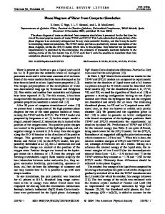
of other solids as well). In other words, the free energy of solids presents important finite size effects. This is further illustrated in figure 4 where the free energy is plotted as a function of 1/N. The estimated value of A/(NkB T ) in the thermodynamic limit from our results is 4.9590(2), which is in good agreement with the estimates of Polson et al. [142] (4.9589), Chang and Sandler [149] (4.9591), Almarza [150] (4.9589) and de Miguel et al. (4.9586) [151] (all obtained from free energy calculations although with different implementations). Therefore, the value of the free energy of hard spheres in the thermodynamic limit for the density ρ∗ = 1.04086 seems to be firmly established. 12.00

4.98 11.50 11.00 *

4.94

p

A/(NkT)

4.96

10.50

4.92 4.90 0

10.00

Exact value FSC-FL

0.002

0.004 0.006 1/N

0.008

0.01

9.50 0

0.01

0.02 1/N

0.03

0.04

Figure 4. Left. Free energies of HS in the fcc solid for ρ∗ = 1.04086 as a function

of system size (filled circles). The open circles represent the free energies after including the Frenkel Ladd finite size corrections (i.e., adding (2/N ) ln N to the free energies of the solid). For all values of N the free energies obtained here (black circles) are in excellent agreement with those reported by Polson et al. [142] and de Miguel et al. [151]. Right. Coexistence pressure of the fluid-solid equilibria of hard spheres as a function of the system size as obtained from free energy calculations (filled circles) or from phase switching simulations as reported by Wilding [12] and Errington [14] (open triangles).

A consequence of the strong N dependence of the solid free energy is that the coexistence pressure p∗ also presents a strong N dependence as illustrated in figure 4. It is of interest to estimate the properties at coexistence in the thermodynamic limit. We found [145], p∗ = p/(kB T /σ 3 ) = 11.54(4), ρ∗s = ρs σ 3 = 1.0372, ρ∗l = ρl σ 3 = 0.9387, and µ∗ = µ/(kB T ) = 16.04. The coexistence pressure is in agreement with estimates by Frenkel and Smit [139] (11.567), Wilding [12] (11.50(9)), Speedy [152] (11.55(11)) and Davidchack and Laird [153] (11.55). The Hoover and Ree estimate (11.70) seems now to be a little bit high. The chemical potential at coexistence obtained here is consistent with the value reported by Sweatman [154] (µ∗ = 15.99 − 16.08) obtained using the self referential methodology to compute fluid-solid equilibria. Although finite size effects are present both in fluid and solid phases, they seem to be more pronounced in the solid (probably due to the coupling between the periodical boundary conditions and the geometry of the solid). In principle one is interested in

CONTENTS

28

properties of the system in the thermodynamic limit rather than for a finite size system. To estimate free energies in the thermodynamic limit one should repeat the free energy calculations for several system sizes and extrapolate to the thermodynamic limit. This is quite involved and time consuming. For this reason it is of practical interest to introduce finite size corrections (FSC) that allow the estimation (although in an approximate way) of large systems free energies, by performing simulations of small systems (something similar to the g(r)=1 approximation [130] used to correct for the introduction of the cut-off). Several recipes have been proposed recently [145]. Here we shall describe one of them, namely the Frenkel-Ladd FSC. Table 1. Free energy of the fcc hard sphere solid at a density ρ∗ = 1.04086.

The value of the different terms that contribute to the free energy in the Einstein molecule and in the Einstein crystal methods, are also shown. All free energies are given in N kB T units. The thermal de Broglie wave length was set to Λ = σ, the hard sphere diameter. N 108 256 1372 2048

/(kT /σ 2 )

ΛE 632.026 632.026 1000.00 1000.00

∆A∗1 0.0172 0.0174 0.0018 0.0018

Einstein molecule A∗0 ∆A∗2 -3.0046 7.8830 -3.0116 7.9254 -3.6862 8.6383 -3.6866 8.6403

Asol 4.896 4.931 4.955 4.955

∆A1 0.0175 0.0175 0.0018 0.0015

Einstein ∆A2 -2.9400 -2.9797 -3.6802 -3.6819

crystal A0 7.8180 7.8929 8.6304 8.6347

Asol 4.895 4.931 4.952 4.954

6.4. Finite size corrections: the Frenkel-Ladd approach. In the original paper of 1984, Frenkel and Ladd (FL) provided an expression for the free energy of the solid (2/N) ln N higher than the correct free energy. That was first pointed out by Polson et al. [142]. In Appendix C the reasons for the appearance of the extra term (2/N) ln N will be described. Thus the FL free energy AFsolL /(NkB T ) is given by: AFsolL /(NkB T ) = Asol /(NkB T ) + (2/N) ln N

(59)

Notice that the term (2/N) ln(N) tends to zero in the thermodynamic limit, and therefore the FL expression is valid in this limit. However, for finite systems the FL expression gives a free energy higher than the true free energy of the system. For a typical system size N =350 the difference between both values is on the order of 0.03NkB T . The interesting issue is that the FL free energies although incorrect (for a certain value of N) are relatively close to the value of the free energy in the thermodynamic limit. This is illustrated in figure 4 for the HS system. For this reason, one may simply view the FL expression as containing an approximate prescription for the finite size corrections, providing free energies closer to the thermodynamic limit than the correct free energies of the system of finite size. Other approximate expressions for the finite size corrections (FSC) have been proposed recently [145].

CONTENTS

29

6.5. The symmetry of the orientational field in Einstein crystal calculations For molecular fluids, the choice of the orientational external field used within the Einstein crystal (or Einstein molecule) simulations should be done with care since this can be a source of methodological errors. The position of the molecule is given by the position of the reference point. Things become simpler if the reference point is chosen in such a way that all elements of symmetry of the molecule contain this point. For instance, a convenient choice for H2 O, NH3 , benzene and N2 are the O, the N, the center of the hexagon, and the geometrical center of the N2 , respectively. Now two orthogonal unit vectors ~a and ~b are attached to the reference point, and these two vectors are sufficient to define the orientation of the molecule (in fact two degrees of freedom are needed to locate the orientation of a unit vector ~a, and just one degree of freedom to locate the vector ~b, which is perpendicular to ~a). Therefore the unit vectors ~a and ~b are a useful way of defining the orientation of the molecule (the Euler angles could be used as well but it is more convenient to use ~a and ~b). For convenience the vector ~b is chosen along the principal symmetry axis of the molecule (the Cn with the highest value of n). When the molecule i stands on its equilibrium position and orientation in the crystal then the vectors ~ai and ~bi adopt the values ~aio and ~bio respectively. Thus the subindex 0 will refer to the orientation of the molecule in the equilibrium lattice position. Let us denote as ψa,i the angle between the vectors ~ai and ~aio and ψb,i the angle between the vectors ~bi and ~bio in an instantaneous configuration. Which expression should be used for the orientational field? The translational part will always be given as in equation (19) for the Einstein crystal approach or as in equation (53) for the Einstein molecule approach. The orientational part will be the same for the Einstein crystal or Einstein molecule approaches. We have already given a convenient expression for the orientational field of a molecule with point group C2v (as, for example, water). Let us now give a convenient expression for other symmetries. For a molecule with a point group of type Cnv a convenient expression for UEin−id,or is : UEin,or =

N X i=1



ΛE,a sin2

nψa,i 2

!

+ ΛE,b

ψb,i π

!2  .

(60)

#

(61)

For a molecule with a point group of type Dnh a convenient expression for UEin−id,or is : UEin,or =

N X i=1

"

ΛE,a sin2

nψa,i 2

!

+ ΛE,b sin2 (ψb,i ) .

For a molecule with point group Oh , a convenient expression [57] for UEin−id,or is: UEin,or =

N h X

i

ΛE,a sin2 (ψa,i,min ) + ΛE,b sin2 (ψb,i,min ) .

i=1

(62)

where ψb,i,min stands for the minimum angle between ~bio and the six vectors connecting the reference point of the molecule with the six octahedral atoms/sites and an analogous definition for ψa,i,min . For a linear molecule only one vector (i.e. vector ~bi ) is needed

CONTENTS

30

and the applied field should be of the form, for a D∞,h : UEin,or =

N h X

i

ΛE,b sin2 (ψb,i ) .

i=1

(63)

For a C∞,v molecule a convenient choice is : UEin,or =

N X i=1



ΛE,b

ψb,i π

!2 

.

(64)

When performing a MC run, it is convenient to introduce two different types of moves, translations and rotations. In a translation move the molecule moves as a whole and there is no change in the orientation of the molecule. Only the change in the translational energy with respect to the reference Einstein crystal (or molecule) needs to be computed. In a second type of move the molecule is rotated in a random direction and angle with respect to an axis passing through the reference point of the molecule. Since the reference point does not change the position under such a rotation, only the orientational energy with respect to the reference Einstein crystal (or molecule needs to be computed). The choice of an orientational field adapted to the symmetry of the molecule as the ones proposed here is highly recommended. When this is done the energy with the external field is invariant to any of the symmetry operations of the molecule. Thus, a standard MC or MD program will provide correct values of the orientational contribution to the free energy. One interesting questions is: is it possible to use an external orientational field that does not reflect the symmetry of the molecule? The answer is : in principle, yes, but you should write a special MC or MD code for that purpose. Special moves should be added where the symmetry operations of the molecule are implemented. For instance for water, one should incorporate the C2 operation that exchanges the positions of the two H atoms. Of course the energy of the molecule with the rest of the system is not affected by this operation. However, the energy of the molecule with the external orientational field may change when the external orientational field does not reflect the symmetry of the molecule (see the interesting paper by Schroer and Monson [51] illustrating this problem for benzene). For this reason, it is by far more convenient and simpler to use an orientational field that respects the symmetry of the molecule (examples for Cnv , Dnh , Oh and linear molecules have been given here). This subtle issue of the symmetry of the orientational field may have been an important source of errors in free energy calculations for molecular fluids. Let us just finish by saying that although we found convenient to have the vectors ~a and ~b orthogonal, other choices (as far as they are not colinear) are also valid and correct. 6.6. Einstein crystal calculations for disordered systems Let us now discuss briefly the case of disordered solids. When implementing the Einstein crystal harmonic springs are incorporated to fix the position (as given by the reference point) and the orientation of the molecules of the system to the equilibrium

CONTENTS

31

configuration. In a disordered solid, there may be many possible “equilibrium configurations” differing in a significant way (not just differing in the labelling of the molecules). Let us just give three examples: Plastic crystals. Molecules with an almost spherical shape tend to form plastic crystals when freezing. In these plastic crystals the reference points of the molecules form a true lattice but the other atoms of the molecule are able to rotate (either with a free or with a hindered rotation) around the reference points. In principle the Einstein crystal methodology described in the previous section can also be applied to determine free energies for plastic crystals [28, 31, 32, 33, 36, 37, 57]. In addition to the translational field, an orientational field is included forcing the molecules to adopt an orientationally ordered solid for large values of the orientational field. Some issues should be taken into account when evaluating the free energy for a plastic crystal phase. At low values of the orientational field very long runs should be performed to guarantee that the molecules are able to rotate. Many values (20-30) of the coupling parameter ΛE should be used to compute the integral of equations (38) or (58) (the orientational contribution to the integrand increases quite rapidly for low values of the orientational field). Finally the absence of phase transitions along the integration path should be checked ( the external field should lead the system from an orientationally disordered solid at low values of coupling parameter to an orientationally ordered solid for large values of the coupling parameter without undergoing any phase transition). Water. In the case of solid water (say ice Ih) while the oxygens are ordered (i.e., they form a lattice) the hydrogens are disordered. However, Bernal and Fowler [155] and Pauling [156] suggested that configurations satisfying the so called Bernal and Fowler rules have the same statistical weight and that configurations violating the Bernal Fowler rules can be neglected. The correct estimate of the experimental residual entropy of ice at 0 K by using these two assumptions was a major achievement. Therefore the free energy of ice is approximated by : A = −kB T ln(ΩAconf iguration ) = −kB T ln(Ω) − kB T ln(Aconf iguration ) (65) where Aconf iguration is the free energy (obtained via the Einstein crystal methodology for a certain configuration satisfying the Bernal Fowler rules) and Ω is the degeneracy. Pauling estimates −kB T ln(Ω) as −kB T ln((3/2)N ). Therefore for ices one computes the free energy for a certain configuration and then adds the Pauling contribution to the free energy. This entropy can also be computed numerically (see for instance the work by Berg and Yang [157]). Notice that when MC or MD runs are performed for a certain configuration of ice satisfying the Bernal Fowler rules, the system remains in this configuration along the run. This is because the time required by the system to jump from a configuration to another (both satisfying the Bernal Fowler rules) is beyond the typical time of a simulation run. equation (65) is useful not only for ice but for other disordered solids as well. In fact it can be applied successfully [158, 159, 32, 160, 38] to tangent dimers, formed by two tangent spheres, where Nagle [161] has estimated Ω, and for fully flexible hard sphere chains [42](where Flory and Huggins [162, 163] have

CONTENTS

32

estimated Ω). Partially disordered phases. In certain cases the system possess disorder but, still certain configurations are more likely than others. Getting the free energy in such a situation is especially difficult. Firstly it is important to sample the configurational space properly to obtain equilibrium configurations of the system representative of the partial disorder. Secondly these configurations will differ in statistical weight, so that it does not seem a good idea to perform Einstein crystal calculations for just one configuration, since its statistical weight is unknown. In this case thermodynamic integration can be a more adequate route. An example of a partially disordered phase is the fcc disordered structure of the RPM model (see discussion on this later on). 7. The machinery in action. III. Obtaining coexistence lines: the Gibbs Duhem integration. Once the free energy of the liquid and the solid has been obtained for a reference state it is relatively straightforward to perform thermodynamic integration to obtain it for other thermodynamic states and locate a coexistence point between two phases (in case where it exists). The Gibbs-Duhem integration allows the determination of the coexistence lines once an initial coexistence point is known. 7.1. Gibbs Duhem integration In the year 1993 Kofke realized that the Clapeyron equation can be integrated to determine coexistence lines [164, 165, 166]. The Clapeyron equation between two coexistence phases (labelled as I and II) can be written as: hII − hI sII − sI dp = = dT vII − vI T (vII − vI )

(66)

where we use lower case for thermodynamic properties per particle. Since the difference in enthalpy and volume between two phases can be determined easily (at a certain T and p) the equation can be integrated numerically. When implementing the Gibbs Duhem integration one obtains the coexistence pressure for the selected temperatures (the temperature acting as the independent variable). This is quite convenient when the coexistence line does not present a large slope in the p − T plane. When the slope of the coexistence line is large within a p − T representation then it may be more ∆v = T∆h . In this convenient to integrate the Clapeyron equation in a different way: dT dp case the coexistence temperatures are determined for a set of selected pressures (the pressure acting as the independent variable). A fourth order Runge-Kutta algorithm is quite useful to integrate the differential equation. It is important to stress that anisotropic NpT simulations should be used for the solid phase within Gibbs Duhem calculations. Isotropic NpT simulations could be used for fluid phases and for solids of cubic symmetry.

CONTENTS

33

7.2. Hamiltonian Gibbs Duhem integration When a coupling parameter λ is introduced within the expression of the potential energy of the system, then a set of Generalised Clapeyron equations can be derived [31, 167, 168]. For two phases at coexistence: gI (T, p, λ) = gII (T, p, λ).

(67)

If the system is perturbed slightly while preserving the coexistence it must hold that: ! ! ∂gII ∂gI dλ = vII dp − sII dT + dλ, (68) vI dp − sI dT + ∂λ ∂λ the last terms appearing in equation (68) are due to the presence of the new intensive thermodynamic variable λ. If λ is constant when performing the perturbation then one recovers the traditional Clapeyron equation. If the pressure remains constant when the perturbation is performed (so that T and λ are changed) then one obtains : T [(∂gII /∂λ) − (∂gI /∂λ)] dT = (69) dλ hII − hI ∂g It is simple to show (within the NpT ensemble ) that ∂g/∂λ is nothing but ∂λ = E D ∂u(λ) , which can be determined within an NpT simulation. The final working ∂λ N,p,T,λ expression of the Generalised Clapeyron equation (for perturbations of T and λ while keeping p constant) is : dT T (< ∂uII (λ)/∂λ >N,p,T,λ − < ∂uI (λ)/∂λ >N,p,T,λ) = (70) dλ hII − hI This Generalised Clapeyron equation can be integrated numerically yielding the change in coexistence temperature (at a certain pressure) due to a perturbation of the Hamiltonian of the system (i.e., of the potential energy). A similar expression can be obtained for the case in which the system is perturbed at constant T (changing the pressure and λ ). In this case one obtains : dp < ∂uII (λ)/∂λ >N,p,T,λ − < ∂uI (λ)/∂λ >N,p,T,λ =− (71) dλ vII − vI The change in the coexistence pressure (at a certain temperature) due to a change in the Hamiltonian of the system (potential energy) is then obtained. Equations (71) and (70) will be denoted as Hamiltonian Gibbs Duhem integration. Hamiltonian Gibbs Duhem integration is a very powerful technique since it allows one to analyse the influence of the parameters of the potential on the coexistence properties. It also allows one to change the parameters of the potential to improve phase diagram predictions. These two possible applications will be illustrated later on for the case of water. In the particular case in which λ is used as a coupling parameter taking the system from a certain potential to another (by changing λ from zero to one): U(λ) = λUB + (1 − λ)UA . Then the generalised Clapeyron equations can be written as: I T (< uB − uA >II dT N,p,T,λ − < uB − uA >N,p,T,λ) = dλ hII − hI

(72)

(73)

CONTENTS

34 I < uB − uA >II dp N,p,T,λ − < uB − uA >N,p,T,λ =− dλ vII − vI

(74)

where uB is the internal energy per molecule when the interaction between particles is described by UB (with a similar definition for uA ). If a coexistence point is known for the system with potential A, then it is possible to determine the coexistence conditions for the system with potential B (it is just sufficient to integrate the previous equations changing λ from zero to one). In this way the task of determining the phase diagram of system B (unknown) from the phase diagram of system A (known) is simplified considerably. 8. Coexistence by interfaces 8.1. Direct fluid-solid coexistence In 1978 Ladd and Woodcock devised a method to obtain fluid-solid equilibria, without free energy calculations, the direct coexistence method [169, 170, 171]. In this method, the fluid and the solid phases are introduced into the simulation box, and simulations are performed (NVE MD) to achieve equilibrium between the two coexistence phases. The coexistence conditions can then be obtained easily. Although the initial results for LJ and inverse twelve power were not very successful (probably due to the small size of the systems and to the short length of the runs), the method is becoming more popular in the last few years. In fact it has been applied to simple fluids [172, 173, 174, 175, 153, 176], metals [177, 178, 179, 180], silicon [181], ionic systems [182, 183], hard dumbells [184], nitromethane [135] and water [108, 109, 185, 186, 187, 188, 189, 190, 191]. Two simulation boxes, having an equilibrated solid and liquid respectively, are joined along the z axis (the direction perpendicular to the plane of the interface). That could generate overlapping at the interface, and this overlapping should be relaxed/removed. The coexistence conditions (i.e., pressure, temperature) will be independent on the plane selected for the interface, but the dynamic behavior (and of course the interface properties) will be different for different planes [192, 193, 190]. The direct coexistence method can be implemented either within Molecular Dynamics or Monte Carlo simulations. Both are equally valid, although if dynamical properties are of interest (for instance crystal growth rates) then MD is the only choice. The direct coexistence method was firstly used in the NVE ensemble , but other ensembles as NV T , NpH, NpT , Npz T can be applied. Each ensemble will have its advantages and disadvantages, and the election of one ensemble or another depends on the information that one wants to obtain. Broadly speaking there are two kinds of ensembles, those at which it is possible to reach equilibrium having two coexistence phases at equilibrium and those for which it is not possible to have two phases at equilibrium. Obviously for the study of interface properties only those ensembles that lead to equilibrium should be used. A. NVE ensemble

CONTENTS

35

This is the simplest approach. The idea behind the method is that the system will evolve to the equilibrium temperature and pressure by moving the interface (so that either the amount of solid or the amount of liquid increases). If the system is above the melting temperature, the solid will melt provoking (at constant E) a decrease of temperature. If the system is below the melting temperature, the fluid will freeze provoking (at constant E) an increase of temperature. In NV E runs the initial configuration should not be too far from equilibrium to guarantee some portion of liquid and solid in the final configuration. The equilibrium temperature and pressure are obtained in NV E simulations at the end of the run. The knowledge of the coexistence pressure only at the end of the run is a serious problem. In fact the lattice parameter used in the xy plane (which remains fixed along the run) may not correspond to the equilibrium value for the solid at the coexistence pressure. In other words, stress was introduced, and that may affect the free energy of the solid and, therefore, the melting point. This can be adjusted by trial an error [172, 153]. B. NVT ensemble In the NV T ensemble the system also evolves to equilibrium by changing the relative amount of liquid and solid phases, in this case to adjust the densities and pressure to their coexistence values. One important difference with the NV E ensemble is that, in the NV T , the heat released or absorbed by the crystallization or the melting is immediately accommodated by the thermostat and, therefore, it is expected that the system will attain the equilibrium faster than in the NV E simulations. Actually, heat transfer is usually the determining rate in the crystallization or melting process, and it has been seen that the presence of a thermostat in the simulations leads to crystallization rates much higher than those measured experimentally [194]. However, as in the NV E case, the solid is not able to relax in the xy plane and, therefore, the system might be under some stress. C. NpH ensemble A less common approach is to perform the simulations in the isobaric-isoenthalpic NpH ensemble [195], with anisotropic scaling, i.e., the three edges of the simulation box change independently (see, for example, Ref. [187]). In this ensemble, the system will also attain the equilibrium, in this case by evolving towards the coexistence temperature. One advantage with respect to the previous ensembles is that now the fluctuations of the volume will allow the solid to relax, removing the presence of stress. Moreover, as the volume of the box is allowed to change, the system can adapt more easily to changes in the relative ratio of the amount of solid and liquid phases, especially when the densities of the solid and liquid phases are very different. The problem in this case is that it is not strictly correct to use simulations under constant pressure in the presence of an interface, because, due to the contribution of the interface, the normal and tangential components of the stress tensor are not equal. However, if the system is chosen to be very large in the direction perpendicular to the interface, it is expected that the error introduced by the presence of the interface will be small. Another disadvantage of this ensemble is that, as in the NV E, the transfer of heat is not very efficient and, therefore,

CONTENTS

36

long simulations are needed to obtain the equilibrium. D. NpT ensemble It is possible to tackle both the problem of having stress in the solid and of slow heat transfer by performing simulations in the anisotropic NpT ensemble where each of the edges of the box changes independently. In this case, as the volume is able to fluctuate, the solid can relax to equilibrium and, as the temperature is fixed, the transfer of heat will occur very rapidly. However, as in the NpH ensemble, the use of the NpT ensemble in the presence of an interface is not strictly correct, although, as mentioned before, it is expected that the error is small for a system sufficiently large along the z axis. One important difference of this ensemble with the previous ones is that, as both the pressure and temperature are set, it is not possible to have the interface at equilibrium. The procedure to determine the coexistence properties is as follows. At a given pressure, different simulations are performed at a few temperatures. If the temperature is above the melting temperature the solid will melt (i.e. the total energy of the system will increase) and on the contrary, if the temperature is below the melting temperature the fluid will freeze (i.e. the total energy will decrease). In this way, it is possible to establish a lower and upper limit to the melting temperature. E. Npz T ensemble We have mentioned before that, due to the contribution of the interface, the stress tensor has different normal and transversal components and, therefore, it is not correct to perform simulations under constant pressure in the presence of an interface. The correct way would be to allow the size of the box to change only along the axis normal to the surface, i.e., the z axis. We will call such ensemble Npz T . The procedure to determine the coexistence properties is completely analogous to the procedure followed in the NpT ensemble. The only difference is that now a new starting configuration with the corresponding bulk lattice parameter at pressure pz and temperature T must be generated for each simulation at different temperature and/or pressure in order to avoid having stress in the solid. This was not necessary in the NpT ensemble, as the fluctuations along the x and y planes allowed the solid to relax to equilibrium. Two issues that deserve special attention when implementing the direct coexistence method are the system size and the length of the simulation. As with regards to the system size, a typical simulation box could have 10 molecular diameters in the x and y direction and about 30 in the z direction. Accordingly, studies by direct coexistence used typically 1000-3000 molecules, and these sizes provide results relatively close to the thermodynamic limit [173, 178, 135, 189, 190]. Besides large system sizes, extremely long simulations are also needed (10 millions of time steps or more may be needed in many systems). Systems without a thermostat (NV E, NpH) may require even longer runs, since heat transfer along the interface may be quite slow.

CONTENTS

37

8.2. Estimating melting points by studying the free surface It is now commonly accepted that melting starts at the surface and, already at temperatures lower than the bulk melting point, solids exhibit a liquid-like layer at the surface [196, 197, 198, 199, 200, 201, 202, 203, 204]. Thus for most substances a liquid layer is presented in the surface even at temperatures below the melting point. When the thickness of this layer diverges at the melting point this is denoted as surface melting. When the thickness of the liquid layer remains finite (or even zero) at the melting point this is denoted as incomplete surface melting [205, 206, 207]. The thickness of the quasiliquid layer for a certain T depends on the considered material and on the exposed plane (as labelled by the Miller indexes). When the size of the liquid layer is sufficiently large either because the system has surface melting or incomplete surface melting (with an significant thickness of the liquid layer) then it is not possible to superheat a solid. This is the reason why experimentally solids usually melt at the melting point (at least one plane of the crystals of the powder presents a large quasi-liquid layer provoking the melting of the whole sample). For instance for ice it is not possible to superheat the solid, except for a few nanoseconds [208]. Superheating of solids (over macroscopic times) has been found experimentally only for monocrystals when the exposed planes have no liquid layer at all. Since for most of substances a quasi-liquid layer will be present at the melting point it is expected that for most of materials, the melting will occur at the melting point (when having a free surface). That provides a remarkably simple methodology to estimate melting points (at zero pressure). NVT simulations of the solid exhibiting a free surface are performed at different temperatures. A convenient geometry is to locate a slab of solid in the center of an orthorhombic simulation box. The pressure will be essentially zero since no vapor was introduced in the simulation box, and besides the vapor pressure is typically so small that the sublimation of a molecule from the solid will be a rare event within the typical simulation times. The lattice parameter of the solid in the direction perpendicular to the interface should correspond to the equilibrium values at zero pressure for the studied temperature. At temperatures below the melting point a stable thin liquid layer will be formed in the surface. At temperatures above the melting point the solid will melt. The simulations should be rather long to allow the system to melt completely. In the case of water, the ice took about 10-20ns to melt in the presence of a free surface. This technique has been applied successfully to estimate the melting point of the LJ model, water [209] and nitro-methane [203, 210]. Notice that the technique will fail, for instance for NaCl, a substance having no liquid layer on the free surface [183]. 9. Consistency checks Evaluation of free energy and coexistence points requires more effort than performing simple NpT runs. Besides, the possibility of introducing errors in the calculations is relatively high. For this reason it is a good idea to introduce several tests to guarantee

CONTENTS

38

the accuracy of the calculations. 9.1. Thermodynamic consistency In a number of cases it is possible to determine the free energy for two different thermodynamic states. For instance for a solid the free energy at two different densities along an isotherm can be determined by using Einstein crystal calculations. The free energy difference between these two states (as obtained from free energy calculations) should be identical to that obtained by thermodynamic integration (integrating the EOS along the isotherm). We indeed recommend the implementation of this test before performing any further calculation. Failing in the test indicates an error in the free energy calculations. However, passing the test it is not a definite proof of the correctness of the free energy calculations. They could still be wrong by a constant (being the constant identical for the two thermodynamic states). It is clear that other tests should also be introduced to guarantee the correctness of the calculations. 9.2. Consistency in the melting point obtained from different routes The melting point obtained from free energy calculations should be similar to that obtained from direct coexistence simulations (where the fluid and the solid phases coexist) within the simulation box. Notice that only fluid-solid equilibria can be studied by direct coexistence (it is not obvious how to implement solid-solid equilibria by direct coexistence). This is indeed a useful test. An incorrect prediction of the free energy of the solid phase (the typical source of errors) will provoke an incorrect prediction of the fluid-solid equilibria as compared to the estimate obtained from direct coexistence techniques. Important differences (above 2-3%) in the melting point estimated from free energy calculations and from direct coexistence are not acceptable. The reader may be surprised by the fact that we stated that both melting points should be similar instead of stating that they should be identical. In the thermodynamic limit (for very large system sizes) they should indeed become identical. However for finite systems some technical aspects may provoke small differences. There are at least two reasons: (a) System size effects. The fluid-solid equilibria may have a strong N dependence. For this reason the coexistence pressure/temperature obtained from free energy calculations for a system of N molecules will not be identical to that obtained from direct coexistence simulations obtained with N ∗ molecules. The case of HS was illustrated in a previous section. In general the stability of the solid increases as the system becomes smaller. Since typically N ∗ > N, then the solid will appear slightly more stable in the free energy calculations than in the direct coexistence results (assuming that no FSC corrections were introduced). This is what one may expect when the only difference between both type of calculations is the size of the system. (b) Cut-off effects. This is important when the cut-off used in free energy calculations is different from that used in direct coexistence simulations. The difference in the melting point may just be due to the fact that we are simulating two sightly

CONTENTS

39

different potentials. Even if the potentials were truncated at the same distance in both methodologies there may be differences. For instance, in free energy calculations, the potential may be truncated at a distance rc , but long range corrections can be incorporated in the calculations [130]. In direct coexistence simulations, the potential may have been truncated at the same rc but in this technique it is difficult to incorporate long range corrections. Therefore certain differences in the melting point between free energy simulations and direct coexistence calculations can be due to a different implementation of the potential. Notice that effects a) and b) may occur simultaneously. For instance in the case of water, different number of particles were used in free energy calculations and in direct coexistence simulations (effect a). But also the truncation of the potential (LJ contribution) was different in the free energy simulations (where long range corrections were included) and in the direct coexistence simulations (where they were not included). In any case for water models we found differences in the melting point as estimated from both techniques of about 1-2% [211, 189]. 9.3. Some useful tests involving Gibbs Duhem integration Some useful tests that can be performed when using the Gibbs-Duhem technique are: • The coexistence lines should be identical (within statistical uncertainty) when the integration is performed forward (say by increasing the T) and when it is performed backward (say by decreasing the T). • If free energy calculations were used to locate an initial coexistence point between phases I-II, I-III and II-III, then the three coexistence lines obtained with Gibbs Duhem integration should cross at a point (the triple point). • If the melting point of two models has been determined by free energy calculations then it is also possible to use Hamiltonian Gibbs Duhem calculations to check that the melting point of model B is obtained starting from the melting point of model A and viceversa. • If the melting point of models A and B is known, then Hamiltonian Gibbs Duhem integration could be performed to estimate the melting point of model C. Both integrations (one starting from A and the other starting from B) should provide the same estimate of the melting point of C. • If two coexistence points between phases I and II are known (either by free energy calculations or by direct coexistence) a Gibbs-Duhem integration starting from one of them should pass through the other one. 9.4. Consistency checks at 0 K At zero temperature the condition of chemical equilibrium (i.e., the equilibrium pressure peq ) between two phases, labelled as phase I and II, respectively, is given by: UI (peq , T = 0) + peq VI (peq , T = 0) = UII (peq , T = 0) + peq VII (peq , T = 0)

(75)

CONTENTS

40

Hence, phase transitions between solid phases at zero temperature occur with zero enthalpy change. This is really useful since it means that phase transitions at 0 K can be estimated without free energy calculations (just computing mechanical properties as densities and internal energies). By performing several NpT simulations where the temperature is reduced up to zero it is possible to obtain the EOS (and internal energy) of each solid phase at 0 K. Then by equating the enthalpy, it is possible to locate phase transitions (at 0 K). This can be used as a consistency check. By performing free energy calculations it is possible to locate the coexistence pressure between two phases (I and II) at a finite non zero temperature. Then, by performing Gibbs Duhem simulations it is possible to determine the coexistence line up to 0 K. The coexistence pressure at 0 K obtained from this long route (free energy calculations+Gibbs Duhem integration) should be identical to that obtained from the short route (estimating the properties of the system at 0 K). This is again a severe consistency check. Although runs at 0 K enable a check to be made on the consistency of phase diagram calculations, they do not allow by themselves to draw the phase diagram of a certain model. Gibbs Duhem simulations can not be initiated from a known coexistence point at 0 K since both ∆H and T are null so that its ratio ∆S, which within classical statistical thermodynamics is finite even at 0 K, can not be determined. 10. A worked example. The phase diagram of water for the TIP4P and SPC/E models. We shall now illustrate how the previously described methodology can be applied to determine the phase diagram for two popular water models: SPC/E [212] and TIP4P [213]. We believe that they illustrate quite well the typical difficulties found when determining by computer simulation free energies of solid phases and phase diagram calculations. The SPC/E and TIP4P models are presented in Table 2 (along with two other recently proposed models TIP4P/Ice [214] and TIP4P/2005 [215]). In these models a LJ center is located on the O atom, and positive charges are located on the H atoms. The negative charge is located at a distance dOM from the O along the H-O-H bisector. Let us now describe briefly some of the simulation details. Table 2. Potential parameters for several water potentials. Notice that the OH

bond length and the HOH angle are different for the SPC/E and TIP4P models.

Model ǫ/k(K) SPC/E [212] 78.20 TIP4P [213] 78.0 TIP4P/2005 [215] 93.2 TIP4P/Ice [214] 106.1

σ(˚ A) qH (e) dOM (˚ A) 3.1656 0.4238 0 3.154 0.520 0.150 3.1589 0.5564 0.1546 3.1668 0.5897 0.1577

CONTENTS

41

10.1. Simulation details In our Monte Carlo simulations, the LJ potential was truncated for all phases at 8.5 ˚ A. Standard long range corrections to the LJ energy were added. The importance of an adequate treatment of the long range coulombic forces when dealing with water simulations has been pointed out in recent studies [216, 217, 218, 219] and it is likely that this is even more crucial when considering solid phases. In this work, the Ewald summation technique has been employed for the calculation of the long range electrostatic forces. The real space contribution of the Ewald sum was also truncated at A. The screening parameter and the number of vectors of reciprocal space considered 8.5 ˚ had to be carefully selected for each crystal phase [130, 139]. For the fluid phase we used 360 molecules. The number of molecules for each solid phase was chosen so as to fit at least twice the cutoff distance in each direction. Three different types of runs were performed: NpT, NVT Einstein crystal calculations and Gibbs Duhem integration. The equation of state (EOS) of the fluid was obtained from isotropic NpT runs, whereas anisotropic Monte Carlo simulations (Parrinello-Rahman like) [124, 125, 126] were used for the solid phases. In the NpT runs, about 40000 cycles were used to obtain averages, after an equilibration period of about 40000 cycles. However longer runs were used for the fluid phase at low temperatures. A cycle is defined as a trial move per particle plus a trial volume change. To evaluate the free energy of the solid, Einstein crystal (NVT) calculations were performed (with fixed center of mass). Also the length of the runs was of about 40000 cycles to obtain averages after an equilibration of 40000 cycles. In the Gibbs Duhem simulations a fourth order Runge-Kutta was used to integrate the Clapeyron equation. In total about 60000 cycles were used to pass from a coexistence point to the next one. When using Hamiltonian Gibbs Duhem integration 5-10 values of λ where used to connect the initial to the final Hamiltonian. In the Gibbs Duhem simulations, the fluid, and cubic solid were studied with isotropic NpT runs whereas the solid phases were studied with anisotropic NpT runs. 10.2. Free energy of liquid water The free energy of the liquid is calculated by integrating the free energy along a reversible path in which the water molecules are transformed into Lennard-Jones spheres by switching the charges off. The free energy of the reference Lennard-Jones fluid is reported in the work of Johnson et al. [220]. The energy (say, for the TIP4P model of water, being the treatment for SPC/E fully equivalent) of the system for a given point of the path, λ, is given by: U(λ) = λUT IP 4P + (1 − λ)ULJ

(76)

where λ varies between 0 (LJ) and 1 (water) along the integration path. Given that ∂A(λ)/∂λ =< ∂U(λ)/∂λ >N V T , the free energy difference between liquid water and the Lennard-Jones fluid is given by: AT IP 4P (N, V, T ) − ALJ (N, V, T ) =

Z

λ=1

λ=0

hUT IP 4P − ULJ iN,V,T,λ dλ.

(77)

CONTENTS

42

where < UT IP 4P − ULJ >N,V,T,λ is an NV T simulation average computed for a given value of λ. The integral is solved numerically (using Gauss-Legendre quadrature) by calculating the integrand at different values of λ. In practice we perform the MC runs starting from λ = 1 and going to λ = 0. The final configuration of a run was used as the input configuration of the next run. The LJ fluid chosen as a reference state has the same LJ parameters (ǫ/kB and σ) as the water model. Therefore, the difference UT IP 4P − ULJ is just the electrostatic energy. Once the Helmholtz free energy, A, is . In this way known, the chemical potential is obtained simply as: kBµT = N kAB T + NpV kB T we have computed the free energy of the liquid at 225 K and 443 K (see table 3). In addition to the total free energy we report the free energy difference with respect to the reference LJ fluid (∆A), the residual free energy for the LJ fluid and the ideal free energy (NkB T (ln(ρΛ3 ) − 1)). In this work, for water, we shall assign the thermal de Broglie wave length to Λ = 1 ˚ A both for the liquid and for the solid phases. Table 3. Free energy of liquid water (Aliquid ) for the SPC/E and TIP4P models

(with qr = qv = qe = 1 ). The residual and ideal contributions to the free energy of the reference LJ fluid are given. The residual term of the LJ fluid as obtained from the EOS of Johnson et al. [220]. The ideal term was obtained (in N kB T units) as ln(ρΛ3 ) − 1 where Λ = 1 ˚ A. The difference in free energy between the reference fluid and the water model ∆A is given. Simulations were performed in the NVT ensemble for the density d. Model SPC/E TIP4P SPC/E TIP4P

T (K) 225 225 443 443

p(bar) 564 743 4010 4280

d(g/cm3 ) 1.05 1.05 1.05 1.05

Aliquid /(N kB T ) -21.82 -19.48 -9.53 -8.58

Ares LJ /(N kB T ) 2.500 2.401 2.856 2.777

Aid LJ /(N kB T ) -4.350 -4.350 -4.350 -4.350

∆A/(N kB T ) -19.97 -17.52 -8.04 -7.01

Let us now present some consistency checks for the free energies. We shall only discuss it for the TIP4P model. We have computed the free energy at 225 K and 443 K for the density d= 1.05 g/cm3 . The free energy difference between both states is A443 K /(NkB T ) − A225 K /(NkB T ) = −8.58 + 19.48 = 10.90. Then we calculated the same difference by means of thermodynamic integration along an isochore (eq. 7), obtaining again 10.90 NkB T . Besides Jorgensen et al. have estimated the free energy for the TIP4P model at p=1bar and T=298 K to be G = -6.1 kcal/mol [221]. Starting from the free energy at 225 K and d= 1.05 g/cm3 and performing thermodynamic integration we obtained -6.09 kcal/mol, which is in excellent agreement with the value of Jorgensen et al. [221]. Instead of using the LJ fluid, it is also possible to compute the free energy of the liquid taking the ideal gas as a reference system. We obtain the free energy of TIP4P water at 240 K and 1.0174 g/cm3 by two different routes. In the first one the TIP4P is transformed into a LJ model. We obtained for the free energy of TIP4P in this state A(240 K,1.0174 g/cm3 )/NkB T = -20.15. In the second route, a supercritical isotherm (T=900 K) is used from zero density to 1.0174 g/cm3 (obtaining using equation (12)

CONTENTS

43

-4.699 for A/NkB T of this intermediate state). Then we integrate along the isochore up to 240 K (with a free energy change computed by equation (7) of -15.434 NKB T ). By adding these two numbers together we obtain A(240 K,1.0174 g/cm3 )/NkB T2 =-20.13 from this second route, in very good agreement with that obtained by the first one. The computation of the free energy using the LJ fluid as a reference system is considerably shorter than using the ideal gas (besides this last route is especially difficult since the parameters of the Ewald sum should be chosen carefully along the supercritical isotherm integration). Values of the free energy of liquid water for other potential models have been reported recently [222]. 10.3. Free energy of ice polymorphs The free energy of the different ice polymorphs is calculated using the Einstein crystal method (with fixed center of mass). The O is used as reference point and the field used is that described by equations (18), (19) and (20). For disordered ices [223, 224, 225] (Ih, Ic, III, IV, V, VI, VII, XII) the oxygens form a well defined lattice, but the water molecules can orient in different ways for a given oxygen lattice provided that the BernalFowler ice rules [155] are satisfied. We have generated the disordered solid structures (with almost zero dipole moment) using the algorithm proposed by Buch et al. [226] (see Ref. [227] for other algorithm). For proton disordered ices we calculated the free energy for a particular proton disordered configuration. Due to the fact that there are many configurations compatible with a given oxygen lattice, there is a degenerational contribution to the free energy. The degenerational entropy of ice was estimated by Pauling in 1935 [156] as Sdeg = kB ln Ω = kB N ln(3/2). Therefore, the disordered ice phases have an extra contribution to the free energy of −NkB T ln(3/2). Ices III and V present partial proton ordering [228], and that decreases a little bit the Pauling estimate[229, 230]. For ices III and V we shall use the sligthly lower value of the degenerational entropy estimated by MacDowell et al.[229]. For ices II,IX,VIII and the antiferroelectric analogous [231] of ice XI the protons are ordered, and there is no degenerational entropy contribution. Generating an initial configuration for proton ordered ices is relatively straightforward. The free energy calculations were performed in the NVT ensemble using the equilibrium shape of the simulation box obtained in anisotropic NpT runs. The location of the springs of the ideal Einstein crystal field were chosen to be close to the equilibrium positions/orientations of the molecules. The computed free energy should not depend on the particular choice of the positions and orientations of the ideal Einstein crystal field (provided that they are sufficiently close to the equilibrium position and orientations of the molecules in the absence of the external field). Several strategies are possible. For instance one could choose the position/orientations of the external field as those obtained from an energy minimisation at constant density (using the equilibrium box shape of the system). Another possibility is to use the experimental crystallographic positions (if available) of the atoms of the molecule and modify them slightly to satisfy

CONTENTS

44

the bond lengths and angles of the model ( the bond lengths may be different in the model and in the real molecule, as for instance in SPC/E water). Also, experimental crystallographic positions (if available) could be used for the reference point (oxygen in the case of water) , and the orientations could be optimised from an energy minimization. We have used this last approach for ices. This approach has also been used recently by Wierzchowski and Monson for gas hydrates [68]. To obtain ∆A2 we used Gaussian integration with 12 points. ∆A1 was evaluated from runs (200000 cycles) of the ideal Einstein crystal with fixed center of mass. The value of ΛE (in kB T /(˚ A)2 ) was identical to the value selected for ΛE,a and ΛE,b (in kB T units). The value of ΛE was chosen so that the computed value of ∆A1 differs by about 0.02NB T units from the lattice energy of the solid (defined as the intermolecular energy of the system when the molecules occupy the positions and orientations of the external Einstein field). Coexistence between phases at 150, 225 and 443 K were investigated. Therefore, the free energy calculations have been performed at those temperatures. In tables 4 and 5 we report the free energy (Asol /(NkB T )) calculated for different ice phases for SPC/E and TIP4P respectively. The different contributions to the free energy (A0 , ∆A1 , ∆A2 ) are given. The term A0 is the sum of ACM Eins−id plus ∆A3 plus a finite size correction (Frenkel-Ladd type, (2/N) ln N). For proton disordered ices the value of Asol is the sum of A0 , ∆A1 , ∆A2 and the Pauling degeneracy entropy −NkB T ln(3/2). For proton ordered ices (XI,II,IX,VIII) the total value of A is just the sum of A0 , ∆A1 , ∆A2 . The lattice energy Ulattice /NkB T is the energy of the solid when all water molecules remain fixed on the position/orientations of the Einstein crystal field (being the value of ∆A1 /(NkB T ) quite close to Ulattice /NkB T ). The free energies of the SPC/E model are lower than those of the TIP4P (this is consistent with their lower internal energies). As a consistency check we determined via Einstein crystal calculations the free energy of ice VI at two different thermodynamic conditions for the SPC/E and TIP4P. Let us discuss the results for TIP4P. For TIP4P (ice VI) we obtained from free energy calculations A1 (225 K,1.480 g/cm3 )=-17.67 NkB T and A2 (150 K,1.498 g/cm3 )=30.65 NkB T (both states having a pressure of 25000bar). Starting from the value of A1 and performing thermodynamic integration we estimated A2 (150 K,1.498 g/cm3 )=30.66 NkB T in excellent agreement with the value obtained from Einstein crystal calculations. 10.4. Determining the initial coexistence points Once the free energy of each phase is known, it is possible to find the points in the pressure-temperature plane at which two phases have the same chemical potential; i. e., the coexistence points. Given that most of the free energies and equations of state were obtained either at temperatures 150 or 225 K and at pressures 500 or 5000 bar, we focus the search of the coexistence points at these temperatures and pressures. Figure 5 shows the chemical potential as a function of the pressure at 150 K for ices Ih, II, and VI. For a given pressure, the phase of lowest chemical potential is the

CONTENTS

45 Table 4. Free energy of the ice polymorphs for the SPC/E model (with qr = qv =

qe = 1). The free energy reported in the last column corresponds to the sum of all the terms (A0 +∆A1 +∆A2 ) plus the degenerational free energy (−N kB T ln(3/2)) for the case of orientationally disordered phases (the typical uncertainty of the resulting solid free energies is about 0.05N kB T ). For ices III and V we did not use Pauling estimate for the degenerational free energy (−N kB T ln(3/2)) since these ices present partial proton disorder, but the slightly lower value reported by MacDowell et al.[229]. The number of molecules used for each solid phase is indicated in parenthesis just after the Roman numeral of the phase. A finite size correction (Frenkel Ladd type) has been included in A0 . The thermal de Broglie wave length Λ was set to Λ = 1 ˚ A. The residual internal energy of the ice U is reported, so that the entropy of the solid can be obtained easily from the relation S = (U − Asol )/T . The orientational contribution to A0 (equation (29)) was computed from the approximate expresion given in Reference [48].

Ice p(bar) Ih(288) 500 Ic(216) 2620 II(432) 5000 III(324) 5000 IV(432) 5000 V(504) 5000 VI(360) 25000 VI(360) 25000 VII(432) 81690 VIII(600) 60000 IX(324) 5000 XI(360) 500

T (K) d(g/cm3) 150 0.965 150 0.983 150 1.269 150 1.229 150 1.353 150 1.316 150 1.492 225 1.474 443 1.700 225 1.743 150 1.244 150 0.971

U N kB T

ΛE ˚−2 (A ) kB T

A0 N kB T

∆A2 N kB T

∆A1 N kB T

Asol N kB T

-46.08 -46.14 -46.42 -44.89 -43.97 -44.39 -43.29 -27.88 -9.79 -23.92 -46.31 -46.26

25000 25000 25000 25000 25000 25000 25000 25000 9000 25000 25000 25000

29.46 29.45 29.47 29.46 29.47 29.47 29.46 29.46 26.40 29.47 29.46 29.46

-16.92 -16.85 -17.27 -19.10 -18.23 -20.11 -19.78 -19.94 -16.58 -19.38 -19.10 -18.01

-48.94 -48.95 -49.08 -45.66 -45.54 -44.17 -42.81 -28.69 -13.81 -24.68 -46.93 -48.08

-36.84 -36.80 -36.91 -35.73 -34.73 -35.23 -33.56 -19.60 -4.41 -14.61 -36.60 -36.65

most stable one. Ice Ih is the stable phase up to 3041 bar. At that pressure, ices Ih and II coexist. Beyond 3041 bar, ice II is the stable phase up to 6215 bar, where the chemical potentials of ices II and VI are equal. For higher pressures ice VI is the stable phase. By performing similar plots, coexistence points between different phases could be determined. In Table 6 these coexistence points are presented (for TIP4P and SPC/E). The relative stability between ices Ih and Ic (or between ices V and XII) could not be determined since the free energy difference between these solids was smaller than the typical uncertainty of our free energy calculations (0.05NkB T ). As to the stability of ices Ih(Ic) with respect to ice XI (we used the antiferroelectric version of ice XI of Davidson and Morokuma [231] rather than the true ferroelectric version), we found that the XI-Ih transition occurs at 84 K for SPC/E and 18 K for TIP4P (being the proton ordered ice XI the stable phase at low temperatures). The region of the phase diagram corresponding to 5000 bar (figure 6) is the most problematic given that there are as many as seven phases competing; namely, ices II,

CONTENTS

46 Table 5. Same as table 4 for the TIP4P model.

Ice p(bar) Ih(288) 1365 Ic(216) 500 II(432) 8230 III(324) 5000 IV(432) 5000 V(504) 5000 VI(360) 25000 VI(360) 25000 VII(432) 78350 VIII(600) 60000 IX(324) 5000 XI(360) 500 XII(540) 5000

T (K) d(g/cm3) 150 0.966 150 0.958 150 1.269 150 1.237 150 1.353 150 1.315 150 1.498 225 1.480 443 1.700 225 1.743 150 1.238 150 0.959 150 1.358

U N kB T

ΛE ˚−2 (A ) kB T

A0 N kB T

∆A2 N kB T

∆A1 N kB T

Asol N kB T

-42.50 -42.50 -41.80 -41.43 -40.86 -41.13 -40.26 -25.91 -8.66 -21.97 -42.25 -42.53 -40.94

25000 25000 25000 25000 25000 25000 25000 25000 9000 25000 25000 25000 25000

29.46 29.45 29.46 29.46 29.47 29.47 29.46 29.46 26.40 29.47 29.46 29.46 29.47

-16.92 -16.96 -16.98 -18.82 -18.18 -19.62 -19.20 -19.58 -16.76 -19.11 -18.85 -17.03 -18.80

-45.55 -45.52 -44.75 -42.63 -42.60 -41.56 -40.48 -27.12 -12.85 -23.24 -42.56 -45.50 -42.20

-33.45 -33.47 -32.28 -32.39 -31.74 -32.11 -30.65 -17.67 -3.63 -12.90 -31.98 -33.09 -31.94

-22

Ih II VI

150 K

-26

-30

Ih -32 0

II

6215 bar

-28

3041 bar

µ(kBT)

-24

VI

1000 2000 3000 4000 5000 6000 7000 8000

p(bar) Figure 5. Chemical potential as a function of pressure at 150 K for ices Ih, II and VI modeled with TIP4P.

III, IV, V, IX and XII and the liquid. For SPC/E, ice II is clearly the most stable phase among the solid polymorphs. The liquid is again the stable phase at high temperatures (beyond 250 K). For the case of TIP4P, ices V and XII are the solid phases of lower chemical potential. The free energy difference between both polymorphs (0.008 NkB T ) is smaller that the error bar (0.05 NkB T ), so we could not determine which one is the most stable. Liquid water coexists either with ice XII or with ice V at 205 K at 5000 bar.

CONTENTS

47 Table 6. Coexistence points for TIP4P and SPC/E models from free energy

calculations (and thermodynamic integration).

Model SPC/E SPC/E SPC/E SPC/E SPC/E SPC/E SPC/E SPC/E SPC/E SPC/E TIP4P TIP4P TIP4P TIP4P TIP4P TIP4P TIP4P TIP4P TIP4P TIP4P TIP4P TIP4P TIP4P

Phases Ih-II II-VI liquid-II liquid-VI VI-VIII liquid-VIII liquid-VII liquid-Ih liquid-Ic liquid-XI liquid-Ih Ih-II II-VI II-V II-III liquid-III liquid-V liquid-VI VI-VIII liquid-VII liquid-Ic liquid-XI liquid-XII

T (K) p (bar) 150 -444 150 25270 250 5000 225 20690 225 57860 225 57500 443 103520 211 500 210 500 187 500 228.8 500 150 3041 150 6215 152.6 5000 180.3 5000 196.6 5000 204.1 5000 225 8940 225 57290 443 91940 228.8 500 192 500 205.0 5000

10.5. The phase diagram of water Once an initial coexistence point has been determined, by using Gibbs Duhem integration (either dp/dT or dT /dp ) it is then possible to draw the complete phase diagram. In certain cases the point where two coexistence lines met (triple point) was used as origin of the third coexistence line emerging from the triple point. The complete phase diagram of SPC/E and TIP4P is presented in figure 7. As can be seen SPC/E fails in reproducing the phase diagram of water (notice for instance that ice Ih is stable for this model only at negative pressures), whereas TIP4P provides a qualitatively correct description of the phase diagram (except for the high pressure region of the phase diagram ). The reason of the failure of SPC/E and success of TIP4P has been identified recently. The low quadrupole moment of SPC/E and the high value of the ratio dipole/quadrupole of this model is the cause of the failure [112, 114]. In fact TIP4P provides a quadrupole moment and a ratio dipole/quadrupole in much better

CONTENTS

48 -26 Liquid II III IV V IX

-34

Liquid II III IV V IX XII

-27 -28

G(KJ/mol)

G(KJ/mol)

-32

-36

-29 -30 -31 -32

-38

-33

160

180

200

220

240

260

160

180

T(K)

200

220

240

260

T(K)

Figure 6. Gibbs free energy versus temperature at 5000 bar for different phases of

SPC/E (left) and TIP4P (right).

10000

VII

p (MPa)

1000

p (MPa)

VIII VI

VI

1000

V

II

liquid III

100

II III

100

I

V liquid

100 150 200 250 300 350 400 450

T (K)

VII

VI 1000

II

liquid

100

I

10

VIII

10000

p+100 (MPa)

VII

VIII

10000

I

10 150 200 250 300 350 400 450

T (K)

10 100 150 200 250 300 350 400 450

T (K)

Figure 7. Phase diagram of water as obtained from experiment (center) and from computer simulations for the TIP4P model (left) and for the SPC/E model (right). The filled circles on the right panel indicate the stability limit of the solid phases in NpT simulations (without interfaces). Notice the shift of 100 MPa in the right panel.

agreement with experiment. The effect of a quadrupole moment on the vapor-liquid equilibria of molecular models is well known [232, 233, 234]. However it seems that the role of the quadrupole on water properties has been overlooked in spite of some warnings about its importance [235, 236, 237, 218, 238, 239]. Figure 7 illustrates how the evaluation of the phase diagram of water by computer simulation is indeed possible. 10.6. Hamiltonian Gibbs Duhem simulations for water The liquid-Ih solid coexistence temperatures at p = 1 bar for TIP4P and SPC/E have been estimated from free energy calculations to be T = 232 ± 5 K and T =

CONTENTS

49

215 ± 5 K, respectively. These numbers are in relatively good agreement with estimates from other authors for TIP4P [22, 23, 187] and for SPC/E [185, 186, 240, 101]. An interesting question is whether these two values (for TIP4P and SPC/E) are mutually consistent. Starting from the SPC/E model and performing constant pressure Hamiltonian Gibbs Duhem simulations (integrating the generalised Clapeyron equation as described previously) one should recover the melting temperature of the TIP4P. In fact starting from the SPC/E ice Ih melting point we obtain T = 232.3 K for TIP4P (see fig.8 ) in very good agreement with the result obtained through free energy calculations. 240

280

270

235

Tfus (Kelvin)

Tfus (Kelvin)

260 230

225

250

240

220

230 From SPC/E to TIP5P From TIP4P to TIP5P

215

210

220

0

0,2

0,4

λ

0,6

0,8

1

210

0

0,2

0,4

λ

0,6

0,8

1

Figure 8. Hamiltonian Gibbs Duhem integration results. Left. Melting temperature of ice Ih as a function of the parameter λ connecting the models SPC/E (λ = 0) and TIP4P (λ = 1). The points were obtained by using Hamiltonian Gibbs Duhem integration. The dashed line is a guide the eye. The horizontal lines correspond to the melting temperatures of SPC/E (dotted line) and TIP4P (dashed-dotted line) as obtained from free energy calculations. Right: Melting temperature of ice Ih for the TIP5P model (λ = 1) obtained from Hamiltonian Gibbs Duhem integration starting from SPC/E or TIP4P models. When connecting two water models by Hamiltonian Gibbs Duhem integration, the position of the oxygen atom and of the HOH bisector was the same in both models.

Once the melting point of ice Ih for TIP4P and SPC/E seems to be firmly established one could use these values to estimate (by using Hamiltonian Gibbs Duhem simulations) the melting point of another water model, as for instance TIP5P [241]. Obviously, the properties of the final model should be independent of the reference model. When the starting model is SPC/E we obtain T = 275 K for TIP5P whereas the calculated result using the TIP4P model as a reference is T = 273 K. The agreement between both estimates is satisfactory taking into account that the error of the GibbsDuhem integration is about 3 K. This is is further illustrated in the right panel of figure 8 which shows the results of the integration. By using Hamiltonian Gibbs Duhem integration the melting point of ice Ih for other models of water was determined. They are presented in Table 7. Notice that most of the water models tend to give low melting points. For models with three charges (SPC, SPC/E, TIP3P, TIP4P, TIP4P/Ew,

CONTENTS

50 Table 7. Melting points obtained from free energy calculations (TIP4P and SPC/E), Hamiltonian Gibbs Duhem integration (rest of the models)[215, 211, 242, 214], and from direct fluid-solid coexistence. The last column is the value of Ts (see text) obtained from simulations of ice Ih with a free interface. TIP4P-Ew is a water model proposed by Horn et al. [243] and NvdE is a six sites model proposed by Nada and van der Eerden [244].

Model TIP4P/Ice TIP4P/2005 TIP4P-Ew TIP4P TIP5P SPC/E NvdE

Free energy Direct coexistence 272(6) 268(2) 252(6) 249(2) 245.5(6) 242(2) 232(4) 229(2) 274(6) 271(2) 215(4) 213(2) 290(3) 288(3) 1.02

Ice Ih (0.1 MPa) 280

Expt

SPC/E

1.01

TIP4P/Ice TIP4P/2005

260

Free surface 271(1) 249(3) 243(2) 230(2) 217(2) -

TIP4P TIP4P−Ew

ρ (g cm-3)

Tm (K)

240

TIP4P

220 SPC/E

200

1.00

SPC TIP4P/2005

0.99

TIP4P/Ice

SPC

180

0.98

160 TIP3P

TIP5P

0.97

140 1.7

1.8

1.9

2

2.1 2.2 QT (DÅ)

2.3

2.4

2.5

2.6

200

250

300

350

T (K)

Figure 9. Left: melting temperature of ice Ih at 1 bar plotted as a function of the quadrupole moment QT (taken from [112]). QT is defined as the value of (Qxx −Qyy )/2 of the quadrupolar tensor, where the x axis joins the two H atoms and the y axis is perpendicular to the molecular plane. Right: density of water at room pressure as a function of temperature as obtained from experiment (filled circles) and from computer simulations of several water models (lines). The open triangles indicate the melting point of ice Ih for each model.

TIP4P/Ice, TIP4P/2005) a correlation between the melting point and the quadrupole moment has been found. This is illustrated in figure 9. It is seen that models with rather low quadrupole moment (TIP3P, SPC, SPC/E) provide rather low melting points. The melting temperature of TIP4P is closer to the experimental value. Motivated by this we have proposed a new modified TIP4P model, with a higher quadrupole moment, able to reproduce the experimental melting point of water. We have denoted this new model as TIP4P/Ice [214]. A second finding was that for three charge models, the temperature at which the maximum in density occurs at room pressure (TMD) is about 20-25 K above

CONTENTS

51

the melting temperature [242, 245]. Experimentally for water, the maximum in density occurs 4 degrees above the melting point. Therefore it is impossible with three charge models to reproduce simultaneously the melting point and the TMD. It is likely that the inclusion of quantum effects and/or polarizability [246, 247, 248, 249, 250, 251, 252] may be needed to reproduce these two properties simultaneously. For this reason we have proposed the TIP4P/2005, which reproduces the TMD of real water better than any other water model proposed so far (see figure9b). An interesting question is to analyze whether these new models still predict correctly the phase diagram of water. By using Hamiltonian Gibbs Duhem integration it is possible to estimate the phase diagram of a certain water model, starting from the phase diagram of another reference model. Thus by using TIP4P as reference, we have estimated the complete phase diagrams for TIP4P/Ice and TIP4P/2005. The obtained phase diagrams are presented in figure 10. As can be seen these models predict quite well the fluid-solid equilibria of water improving the predictions of TIP4P. The TIP4P/2005 yields also an excellent prediction of the vapor-liquid equilibria. 1000

750 TIP4P/Ice TIP4P/2005 TIP4P

Exptl TIP4P/Ice TIP4P/2005 TIP4P

650

800

550

600

T (K)

p (MPa)

VI

V

450 400 II

liquid

III

350

200 Ih 0 160

180

200

220

240

250 260

280

300

0

0.2

0.4

ρ(g/cm3)

0.6

0.8

1

T (K)

Figure 10. Phase diagram for the TIP4P family. a) Left panel: fluid-solid equilibria (the lines show the predictions for several TIP4P-like models and the symbols represent the experimental data). b) Right panel: vapor-liquid equilibria (the symbols show the predictions for TIP4P-like models and the lines represent the experimental data).

10.7. Direct coexistence simulations To estimate the melting point of ice Ih for several water models by direct coexistence, NpT simulations were performed with 870 molecules and the MD program Gromacs [253, 254]. In the initial configuration half of them formed ice, and the other half were in the liquid state. Both phases were in contact so that these are direct coexistence simulations. The evolution of the energy for the TIP4P/2005 model with time is presented in fig.11. As can be seen the energy increases with time for T = 252, 254, 256 K reaching a plateau (the plateau indicates the complete melting of the ice). The energy decreases for

CONTENTS

52 -42 258 K

252K

252 K

-44

254 K

256K

-46

TIP4P/2005 -48

E(kJ/mol)

-1

E (kJ mol )

-44

TIP4P/2005 -46

242 K

-48

-50 0

2000

4000

t (ps)

6000

8000

245K

0

2000

4000

6000

8000

t (ps)

Figure 11. a) Left panel. Evolution of the total energy (per mole of molecules) in N pT MD simulations of a box containing ice and liquid water at 1 bar for the TIP4P/2005 model. b) Right panel. Total energy as a function of time obtained at several temperatures by performing MD simulations of TIP4P/2005 for a block of ice Ih with a free surface.

T = 242 K reaching a plateau (the plateau indicates the complete freezing of the water). Snapshots of these final configurations can be found in Ref. [189]. At a temperature of 249 K the energy does not change with time, and the interface is stable after 10ns. Therefore this is the estimate of the melting point by direct coexistence for TIP4P/2005. Similar runs were performed for other water models. In Table 7 the melting points of different water models as estimated from direct coexistence are compared to those obtained from free energy calculations. The agreement between both techniques is quite good. Direct interface simulations have been used by several authors to estimate melting points or ice growth rates for different water models [92, 255, 194, 256, 187, 192]. 10.8. Melting point as estimated from simulations of the free surface In figure 11 the evolution of the total energy of ice Ih (having a free surface) with time is presented [209]. At high temperatures, the total energy of the system increases continuously and then reaches a plateau (that corresponds to the complete melting of the solid). The behaviour at low temperatures is different. At the beginning (first 12ns), there is an increase of the energy but after that the energy remains approximately constant, apart from the thermal fluctuations. The analysis of the configurations of the TIP4P/2005 at T = 245 K, shows that the increase of energy during the first 1ns is due to the formation of a thin liquid layer at the surface of ice, which may indicate the onset of surface melting, mentioned already in the Introduction, and first proposed by Faraday [257]. The formation of a quasi liquid layer on the surface of ice below Tm has been found both in experiment (see [258, 259, 260, 261, 262] and references therein) and in computer computer simulation for several potential models of water [263, 264, 265, 266, 92] and it has been explained by several theoretical treatments [258, 260]. By repeating the

CONTENTS

53

simulation at several temperatures it is possible to determine the lowest temperature at which the block of ice melts T+ , and the highest temperature at which it does not melt T− . By taking the average of these two temperatures we obtain what we call Ts = (T+ + T− )/2. Ts provides an estimate of the melting point. The values of Ts obtained for water models are presented in Table 7. As can be seen, Ts is identical to Tm , within the error bar. Thus for ice Ih, the presence of a free surface suppresses superheating and ice melts at the equilibrium melting temperature (although runs of about 10ns or longer may be needed). In figure 12 the final configuration (after a 8 ns

Figure 12. Instantaneous configuration of the TIP4P/Ice system at T = 268 K at the end of a 8ns run. Although the temperature is well below the melting point of the model, a quasi-liquid layer is clearly present in the ice-vacuum interface.

run) obtained for the TIP4P/Ice at a temperature well below the melting point of the model (T = 264 K). As can be seen, a quasi liquid layer is already present in the system. 10.9. Properties at 0 K

Table 8. Residual internal energy (in Kcal/mol) of several ice polymorphs at T = 0 K and p = 0 for popular water models. The results for the most stable phase of each model are presented in bold.

Ice Ih II III V VI

TIP4P/Ice -16.465 -16.268 -16.140 -16.049 -15.917

TIP4P/2005 SPC/E -15.059 -14.691 -14.847 -14.854 -14.741 -14.348 -14.644 -14.169 -14.513 -13.946

TIP5P -14.128 -14.162 -13.320 -13.101 -12.859

In Table 8 the residual internal energies at zero T and p are given for the TIP4P/Ice, TIP4P/2005, SPC/E and TIP5P models. For TIP4P/Ice and TIP4P/2005 ice Ih is the structure with the lowest energy (probably ice XI which is a proton ordered version of ice Ih would have an slightly lower energy but it was not considered for this study). However for SPC/E and TIP5P the lowest internal energy corresponds to ice II. Thus, for

CONTENTS

54

TIP4P/2005 and TIP4P/Ice ice Ih is the stable phase at zero pressure and temperature whereas for SPC/E and TIP5P the stable phase is ice II. From the properties at 0 K it is simple to locate the Ih-II transition pressure at 0 K (see [267]). In figure 13 the predicted pressures using the calculations at 0 K are presented (circles). The lines represent the results obtained from free energy calculations (used to obtain an initial coexistence point at 150 K) and Gibbs Duhem integration. It may be seen that both sets of calculations agree quite well so both sets of results are mutually consistent (i.e., the estimated coexistence pressure at 0 K is the same). It is clear that ice II is more stable than ice Ih at zero temperature and pressure for the SPC/E and TIP5P models. This example illustrates how 0 K properties can be used to test for self consistency in phase diagram predictions. They are also quite useful to test the performance of water models [268, 89, 90, 269, 267]. 300 TIP4P/2005 TIP4P/ICE

p (MPa)

200

100

0 TIP5P

-100 SPC/E -200 0

50

100

150

200

T (K)

Figure 13. Coexistence lines between ices Ih and II as obtained from Gibbs-Duhem simulations for TIP4P/2005, TIP4P/Ice, SPC/E and TIP5P models (solid lines). The symbols represent the coexistence pressures as obtained from the properties of the systems at zero temperature. For each water model, ice Ih is the stable phase below the coexistence line (low pressures) and ice II is the stable phase above the coexistence line (high pressures).

11.

Phase diagram for a primitive model of electrolyte

Let us now present another example of a phase diagram calculation for a completely different model, the restricted primitive model (RPM). The restricted primitive model (RPM) is one the simplest model of electrolytes. It this model the cations are represented by hard spheres of diameter σ having a charge +q and anions represented by hard spheres of diameter σ having a charge −q. The model is quite simple and for this reason it can also be studied theoretically [270, 271]. The system has vapor-liquid equilibrium [272, 273, 274] (in spite of the absence of dispersive forces). Several solid structures can

CONTENTS

55

be considered [275], the simplest being the CsCl like structure (a bcc type of structure with the anions occupying the vertices of a cube and the cations occupying the center of the unit cell). Another possible structure is the fcc disordered structure. In this structure the ions occupy an fcc lattice, but with positional disorder (cations and anions occupy the lattice points in a disordered way). At low temperatures it is possible to conceive a solid structure with an fcc arrangements of the ions, but with positional order. The symmetry of the phase is tetragonal. This phase will be labelled as the tetragonal phase [49]. It is presented in figure 14. Free energy calculations (Einstein crystal) were performed to determine the free energy of the CsCl and tetragonal structures. Due to the presence of partial disorder the Einstein crystal method can not be applied directly (to a snapshot) to get the free energy of the fcc disordered structure (although one may suspect that an strategy similar in spirit to that proposed for the plastic crystal phases can be also successful here if the external field is able to lead the system from disordered configurations to an ordered solid without crossing first order transitions). The RPM system becomes a hard sphere at infinitely high T for which the free energy is known (a trivial mixing contribution should be added). For this reason the free energy of the fluid and of the fcc disordered solid can be obtained by thermodynamic integration. Exchange moves (where a cation and an anion exchange their positions) were used to sample correctly the disorder, both in the fluid and in the fcc disordered structure. 0.4

fcc disordered

0.35 0.3

fluid

T*

0.25 0.2

fcc ordered

0.15 0.1

CsCl 0.05 0 0

0.2

0.4

0.6

0.8

1

1.2

1.4

ρ∗

Figure 14. Left: Tetragonal ordered structure of the RPM model. The atoms form an fcc structure, but the ions are ordered. Right: Phase diagram of the RPM model showing the equilibria between vapor and liquid (inverted triangles), fluid and CsCl like structure (filled circles), CsCl like structure and tetragonal (fcc ordered) phase (rhombs), fluid and tetragonal structure (open circles), fluid and fcc disordered structure (triangles), and ordered-disordered fcc phases (squares).

After computing the free energies, some initial coexistence points were determined, and then by using Gibbs Duhem integration the complete phase diagram was computed. The resulting phase diagram [276, 277, 49, 50] is presented in figure 14. At

CONTENTS

56

high temperatures, freezing leads to the substitutionally disordered close packed structure. By decreasing the temperature this solid structure undergoes an orderdisorder transition transforming into the tetragonal solid. At low temperatures freezing leads to the caesium chloride structure (CsCl) which undergoes a phase transition to the tetragonal structure at high pressures. The tetragonal solid is the stable solid phase at low temperatures and high densities. In a narrow range of temperatures coexistence between the fluid and the tetragonal solid is observed. Three triple points are found for the model considered: the usual vapor-liquid-CsCl, the fluid-CsCl-tetragonal and the fluid-fcc disordered-tetragonal triple point (notice on figure 14 the narrow range of the fluid- tetragonal solid coexistence line). Although initially conceived to describe electrolytes and ionic salts, the RPM has been found to be quite useful to describe certain colloidal mixtures, consisting in equimolar mixtures of colloidal particles of equal size, but with charges of different sign. Thus a colloidal version of the RPM exists [278]. For these colloidal mixtures, three different solid phases have been found experimentally, the fcc disordered solid, the CsCl solid, and a fcc ordered structure [279, 280]. The fcc ordered structure was found to be of CuAu type, rather than the tetragonal structure of figure 14. This difference with the RPM phase diagram seems to be due to the fact that in colloidal mixtures the interaction between charged particles is of Yukawa type rather than being purely Coulombic. This is so because the interaction between charged particles is screened by the presence of an ionic atmosphere due to the counter ions of the colloids. In fact, when this screening is incorporated in the potential with a Yukawa type model, the CuAu structure was found to be stable in a thermodynamic region between the CsCl and the tetragonal structure [56, 281]. In summary the RPM has proved to be quite useful in the description of mixtures of charged colloidal particles. It would be of interest to determine the phase diagram for a model where the two spheres of the model present different size. This is usually called the primitive model. In fact the primitive model (where cations and anions have different size) may indeed be a more general model than RPM, since in real ionic fluids the size of the ions is usually different. A colloidal realization of the PM model has been obtained experimentally [279]. Finally, there is an increasing interest in determining the properties of ionic liquids. It would be of interest to determine the factors affecting the melting point of ionic liquids [282] which are regarded as new solvents. [283]. Work in this direction has appeared recently [284]. 12. Phase diagram of a simplified model of globular proteins A final example of the application of the techniques described here is provided by the calculation of the phase diagram of a simple model of globular proteins. During the last few years there has been an increasing number of studies of the phase behaviour of globular proteins using very simplified models. The first studies have been performed using short ranged isotropic potentials and, even with these very simple models, it was

CONTENTS

57

already possible to reproduce some of the features of the phase diagram of proteins, e.g., the existence of a metastable critical point [285]. However, proteins are known to form very low density crystals, with densities below those of the close-packed crystals typically formed by isotropic potentials, which is indicative of highly directional interactions [286]. Further evidence of the importance of anisotropy in the interactions among proteins has been recently obtained in a theoretical study of the fluid-fluid equilibria. This study has shown that a quantitative agreement with experiments is obtained by the introduction of anisotropy [287], as opposition to isotropic models that only provided a qualitative description. Moreover, theoretical studies of the phase behaviour of anisotropic models are also acquiring much interest due to the fact that several experimental groups have recently been able to produce colloids that are anisotropic either in shape or in their interactions [288, 289, 290, 291]. So far there has been already a few theoretical studies of the phase behaviour of simple anisotropic models [48, 292, 293, 294, 295, 58, 296, 297], although most of them were concerned with the fluid-fluid equilibria rather than with the solid-fluid and solid-solid equilibria. We have used a very simplified model which consists of a repulsive core (the Lennard-Jones repulsive core), plus an attractive tail modulated by Gaussian functions located at some given positions or patches, which will be specified by some vectors. The total energy between two interacting particles will be given by [298, 299, 57]: V (rij , Ωi, Ωj ) =

  VLJ (rij ) V

rij < σLJ

rij , Ωi , Ωj ) LJ (rij )Vang (b !

rij ≥ σLJ

θl2min ,ji θ2 ,ij exp − Vang (rbij , Ωi , Ωj ) = exp − kmin 2 2 2σpatchy 2σpatchy

!

,

(78) (79)

where VLJ is the Lennard-Jones potential, σpatchy is the standard deviation of the Gaussian, θk,ij (θl,ji ) is the angle formed between patches k (l) on atom i (j) and the interparticle vector rij ( rji), and kmin (lmin ) is the patch that minimises the magnitude of this angle. The interaction is a maximum when both patches are pointing at each other along the interparticle vector rij and it will decrease as the particles deviate further from this equilibrium orientation. We have chosen to study a model with 6 patches distributed in an octahedral symmetry. A relatively narrow width of the patches (σpatchy =0.3 radians), for which it is expected that the low density simple cubic (sc) crystal becomes stable. Besides the sc crystal in which each of a particle’s patch is pointing at each one of its six nearest neighbours (see figure 15), there are other three solid phases that might be formed with this model and at this patch width, σpatchy = 0.3 radians. The first structure is a body centred cubic (bcc) solid, in which each patch is aligned with the second neighbours. This structure can be also seen as two interpenetrated sc lattices that almost do not interact between each other (similar to the behavior of high density ice polymorphs). Therefore, a higher density crystal is obtained with a low penalty in the energy. At high pressures it is expected that a closed packed face centred cubic (fcco) structure will also appear. In this case the patches will be also pointing to the

CONTENTS

58

second neighbours. This structure exhibits a much higher energy than both the sc and the bcc solids. Finally, at high temperatures, it is expected that a plastic phase will also appear (fccd), i.e., a solid where the center of mass of each particle is located at the lattice positions of a fcc structure, but that is orientationally disordered.

fluid

fccd

bcc sc

fcco

Figure 15. Left: Phase diagram of the octahedral six-patches model. Labels show the region of stability of each phase. The dashed line in the fluid-sc coexistence region signals the expected fluid-fluid binodal (see Ref. [57] for more details). Right: Structure of the low density sc solid for the octahedral anisotropic model.

Following the procedure described before, the coexistence point between two phases was computed by imposing the conditions of equal temperature, pressure and chemical potential. The free energy of the fluid was computed by thermodynamic integration. In the case of the fluid, the equation of state was integrated up to very low densities, where the fluid can be considered to behave as an ideal gas. The free energy of the solid was computed by Einstein crystal calculations. Once that a coexistence point is known the whole coexistence line have been traced using the Gibbs-Duhem method. The resulting phase diagram is plotted in figure 15. At high temperatures the fluid freezes into the orientationally disordered plastic crystal phase (fccd), at intermediate temperatures into the bcc solid and at low temperatures into the sc crystal. The sc structure is destabilised at high pressure by the bcc solid and, at even higher pressures, the ordered fcc solid becomes stable (fcco). This fcco ordered solid transforms into a plastic crystal fccd as the temperature increases. There are three triple points in the phase diagram: the fluid-sc-bcc, fluid-fccd-bcc and bcc-fccd-fcco. Finally, it is also worth noting that in the neighbourhood of the fluid-sc-bcc and fluid-fccd-bcc triple points, reentrant melting occurs. Coexistence points from free energy calculations were found to be in agreement with those found from direct coexistence calculations. In summary, even for a relatively simple model potential, we have obtained a complex phase diagram with many solid phases and unusual behaviour such as reentrant melting. But the most interesting finding is that even with a very simple model as the one described here, it is possible to reproduce two important features of the phase diagram of globular proteins, namely, the existence of a metastable critical point and the stabilisation of a low density crystal. Similar behavior has been found for a primitive

CONTENTS

59

model of water [146, 48, 300]. Studies of nucleation of these models can be very relevant to understand the crystallization of globular proteins. 13. Conclusions In this work we have reviewed the methodology of free energy calculations and given examples of recent work on the determination of fluid-solid and solid-solid equilibria by computer simulations. Free energy calculations are used to compute initial coexistence points between phases, and then Gibbs Duhem integration is used to compute coexistence lines. Other procedures to estimate fluid-solid equilibria as direct coexistence and simulations of the free surface of the solid have been discussed. The Einstein crystal methodology and the Einstein molecule approach have been presented in a rather comprehensive way. Both methodologies yield identical values of the free energy. It is shown that the free energy presents a strong N dependence, and that finite size corrections are needed to estimate properties of solids in the thermodynamic limit. The issue of the symmetry of the orientational field in Einstein crystal calculations for molecular fluids has been discussed. We do hope that the extensive discussion of all these aspects helps other researchers in the area to perform free energy calculations and phase diagram determination. In fact there are at least six areas where one can predict intense activity in the future. The first one is the determination of the phase diagram of molecular fluids. In this work, the procedure to obtain free energies for water is presented. Besides, free energies and coexistence points for SPC/E and TIP4P models of water are presented by the first time. These results lead to the determination of the full phase diagram for water, performed recently by our group [110]. The example of water illustrates clearly that phase diagram calculations for molecular fluids is indeed feasible nowadays and that it can help to improve current models. In fact these free energy calculations led to the proposal of an improved version of TIP4P denoted as TIP4P/2005. This model is able to describe correctly the phase diagram of water, the maximum in density of water, the density of the ice polymorphs including the methane hydrate [301, 302, 303], the vapor-liquid equilibria [304], the surface tension [305], the diffusion coefficient, and the structure of water [215, 306] over a wide range of temperatures and pressures. The determination of the phase diagram of TIP4P was a crucial step in the development of TIP4P/2005. We do not see any difficulty in performing similar studies to improve potential models for other molecular fluids. The work on water, shows that melting points obtained from free energy calculations, direct coexistence simulations and free surface simulations, are almost identical (taking into account the statistical uncertainties and the slightly different implementations of the potential). The second area where phase diagram calculations can be useful is in the study of ionic systems. Here we reviewed the phase diagram of the RPM model, but it is clear that it would be of great interest the determination of the phase diagram of PM models and of other models of salts (including probably ionic liquids which are becoming increasingly important from a technological point of view). Some ionic systems can also

CONTENTS

60

be used to describe charged colloids. The third area is the area of crystallization of proteins. It is now clear that models with short range anisotropic forces can be regarded as primitive models of proteins. In such models the liquid-liquid separation is metastable with respect to freezing, and the competition between phase separation and crystallization is of great interest to understand the presence or absence of crystallization in proteins. The fourth area is the study of freezing under confinement due to the interest in understanding fluidsolid equilibria on the nanometer scale [307, 308, 309]. The fifth area is the study of the solubility of salts(or solids in general) in water (or solvents in general) where the knowledge of the chemical potential of the solute in the solid phase is required. Very little effort has been devoted to this problem [143, 147]. Finally studies on nucleation [120] should be benefit from the knowledge of the equilibrium melting temperatures. In summary, the study of fluid-solid and solid-solid equilibria of molecular and complex systems by computer simulation is now feasible, and the procedures to do it seem well established. The study of fluid-solid and solid-solid equilibria by computer simulation can play a central role in developing potential models for condensed phases and for providing molecular understanding of a number of phenomena involving solid and liquid phases. The enormous sensitivy of phase diagrams to interaction potentials allows to test the performance of the different potentials available for a certain substance, and offers a unique opportunity for their improvement. 14. Appendices 14.1. Appendix A. Partition function of the Einstein crystal with fixed center of mass The translational contribution to the partition function of an Einstein crystal with fixed center of mass is: QCM Ein,t

=

Z

"

1 h3(N −1)

exp −βΛE

N X

Z

"

#

N X p2i δ( pi )dp1 ...dpN exp −β i=1 i=1 2mi

(ri − rio )

i=1

2

#

N X

δ(

N X

µi (ri − rio ))dr1 ...drN .

(80)

i=1

The integral over the space of momenta is not relevant to compute the free energy and, therefore, we will leave aside this contribution, that we will include simply as a factor P CM : P CM =

1 h3(N −1)

Z

"

#

N X p2i δ( pi )dp1 ...dpN exp −β i=1 i=1 2mi

(81)

#

(82)

N X

We will focus on the integral over the configurational space: CM ZEin,t

=

Z

"

exp −βΛE

N X i=1

(ri − rio )

2

δ(

N X

µi (ri − rio ))dr1 ...drN .

i=1

This integral can be expressed in a simpler way by defining a change of variable, ′ ri − rio = ri . The Jacobian of this change of variable is 1, and the configurational

CONTENTS

61

integral can be written as: CM ZEin,t

=

Z

"

N X

exp −βΛE

′

(ri )

2

i=1

#

δ(

N X

′

′

′

µiri )dr1 ...drN .

(83)

i=1

The Dirac delta function can be written [310] as: N X

"

Z

1 δ( µi ri ) = (2π)3 i=1 ′

N X

exp ik

′

µi ri

i=1

!#

dk,

(84)

the configurational integral can be written as:

" !# N X ik 1 Z ′ 2 ′ ′ ′ (ri ) − = exp −βΛE µiri dkdr1 ...drN . 3 (2π) βΛE i=1

CM ZEin,t

Each term in the summation can be rewritten in a more convenient form: i2 k 2 µ2 i2 k 2 µ2 2ik ik ′ ′ ′ ′ µiri = (ri )2 − µi ri + 2 2i − 2 2i (ri )2 − βΛE 2βΛE 4β ΛE 4β ΛE ikµi ri − 2βΛE ′

=

!2

+

k 2 µ2i 4β 2Λ2E

(85)

(86) (87)

Notice that in equations (84-86) there is an implicit scalar product between the vector k and the accompanying vector. The integral can then be expressed as: CM Zein,t



Z

1 = (2π)3

N X



ikµi  r − exp −βΛE i 2βΛE i=1 ′

!2



k 2 µ2 ′ ′ + 2 i2  dkdr1...drN 4β ΛE

(88)

It is now convenient to do another change of variable: ikµi ′′ ′ (89) ri = ri − 2βΛE To compute the Jacobian associated to this transformation, we will consider the simple case of a system in one-dimension and with two particles. The Jacobian J is given by the following determinant:

J=

J=





′

∂r1 ′′ ∂r1 ′ ∂r2 ′′ ∂r1 ∂k ′′ ∂r1

′

∂r1 ′′ ∂r2 ′ ∂r2 ′′ ∂r2 ∂k ′′ ∂r2



′

∂r1 ∂k ′

∂r2 ∂k ∂k ∂k

1 0

0 1

−2βΛE iµ1

−2βΛE iµ2

(90)

0 0 1



=1

(91)

After applying the change of variable, the integral can be expressed as: CM ZEin,t

1 = (2π)3

Z

"

exp −βΛE

N X i=1

k 2 µ2 (ri ) + 2 i2 4β ΛE ′′

2

!#

′′

′′

dkdr1 ...drN

(92)

This integral can be split in two Gaussian integrals: CM ZEin,t

1 = (2π)3

Z

"

exp −βΛE

N X i=1

′′

(ri )

2

#

′′

′′

dr1 ...drN

Z

"

exp −

k2

PN

i=1

4βΛE

µ2i

#

dk

(93)

CONTENTS

62

whose solution is: CM ZEin,t

1 = (2π)3

π βΛE

!N 3/2

4βπΛE PN 2 i=1 µi

!3/2

(94)

Doing a bit of algebra it can be shown that: CM ZEin,t

=

βΛE π

!3/2

π βΛE

!3(N −1)/2

π βΛE

!N 3/2

N X i=1

or, more simply: CM ZEin,t

=

N X

µ2i

i=1

µ2i

!−3/2

!−3/2

(95)

(96)

Summarising, we have obtained that the partition function of an Einstein crystal with fixed center of mass is given by: QCM Ein,t

=P

CM

π βΛE

!3(N −1)/2

N X i=1

µ2i

!−3/2

.

(97)

When all molecules are identical the reduced mass µi is simply 1/N. Therefore the previous equation can be simplified to: QCM Ein,t

=P

CM

π βΛE

!3(N −1)/2

(N)3/2 .

(98)

which is the final expression for the free energy of an ideal Einstein crystal with fixed center of mass. An explicit expression for P CM is not needed to get the free energy of the solid since it cancels out with a similar term in equation (46). However, it is not difficult to obtain P CM by realizing that equation (81) is formally identical to equation (82) (with µi = 1 and ΛE = 1/(2mi ) and ommiting the prefactor h3(N −1) ). A derivation similar to that used to get equation (96) from equation (82) leads to: 1 (99) P CM = 3(N −1) N −3/2 Λ to be compared with 1 P = 3N (100) Λ so that the ratio P CM /P adopts the value Λ3 N −3/2 . If equation (99) is replaced into equation (98) one obtains: QCM Ein,t

=

1 Λ3(N −1)

π βΛE

!3(N −1)/2

which is dimensionless as it should be.

(101)

CONTENTS

63

CM 14.2. Appendix B: Computing UEin within a Monte Carlo program

The condition of fixing the center of mass of the reference points is quite useful since it eliminates any divergence of the integrand of equation (39). A displacement d~ of a ~ given molecule must be accompanied by a displacement (−d/(N)) of all the molecules of the system (assuming all particles are identical), so that the center of mass remains in its original position. In practice, this is not very convenient. It is more convenient to perform a simulation without the restriction over the center of mass but keeping track of the position of the center of mass [139]. Let us denote as rio the initial position of the reference point of molecule i in the perfect lattice, and ∆RCM is the difference between the present position of the center of mass and its initial position. Let us denote by rUi the actual position in the simulation (without the restriction in the center of mass) of the reference atom of molecule i. Let us define ∆ri = rUi − rio − ∆RCM . Let us compute the energy change when in a trial move, the random displacement of molecule is ∆i . The energy of the old (prefix old) and new (prefix new) configurations is given by: CM,old UEins /ΛE

2 = (∆rold i ) +

X

2 (∆rold j )

j6=i

CM,new UEins /ΛE

= =

rU,old i ∆rold i

+ ∆i − rio − ∆i + ∆i − N

∆Rold CM

!2

+

X

∆i − N

!2

∆rold j

j6=i

+

X

rU,old j

− rjo −

∆Rold CM

j6=i

∆i − N

!2

∆i − N

(102)

We have assumed that all particles have the same mass, so that a displacement ∆i of one of them leads to a displacement ∆i /N of the center of mass. We have not included the orientational contribution since it cancels out when computing the energy change (i.e., the orientational energy is not affected by the translation of molecule i). Therefore, the potential energy change will be given by: N∆i − ∆i CM old ∆i ∆UEins /ΛE = 2∆rold + i .∆i −2∆ri . N N

!2



∆i +  N j6=i X

!2



∆i  (103) − 2∆rold j N

This equation can be simplified since, as the center of mass is constrained, it holds that PN i=1 ∆ri = 0 (in the right hand side, the second and last terms cancel out):

CM ∆UEins /ΛE

=

2∆rold i .∆i

N∆i − ∆i + N

!2

+

X j6=i

∆i N

!2

.

!2

(104)

It is easy to show that this expression can be also written as:   CM old 2 N −1 ∆UEins /ΛE = 2∆ri .∆i + ∆i (105) N In this way, it is possible to perform a MC simulation without keeping the center of mass fixed, but including this constraint through the Monte Carlo acceptance rule.

CONTENTS

64

14.3. Appendix C. The Frenkel-Ladd expression In 1984 Frenkel et Ladd derived an expression for the free energy of a solid. It is not the same as that given by Polson et al. [142] and presented also in this paper. The reason of this difference is the following: • 1. The expression used for ∆A3 by Frenkel and Ladd was (1/N) ln N (in NkB T units) lower than the correct one. • 2. The expression used for ACM Ein−id by Frenkel and Ladd was (3/N) ln N (in NkB T units) higher than the correct one. Taking into account both contributions it turns out that the Frenkel Ladd expression gives an energy (in NkB T units) (2/N) ln N higher than the correct one. Let us describe briefly the source of these two discrepancies. For ∆A3 Frenkel and Ladd used : CM ∆AF3 L = Asol − ACM /P ) − ln(V )) sol = kB T (ln(P

(106)

CM ∆A3 = Asol − ACM /P ) − ln(V /N)) sol = kB T (ln(P

(107)

instead of :

which is the expression to be used when all permutations, N!, are included in the reference ideal Einstein crystal. The second discrepancy is due to the fact that the constraint of fixing the center of mass was implemented by Frenkel and Ladd as : N X

(ri − rio ) = 0

(108)

N X

µi (ri − rio ) = 0

(109)

i=1

instead of :

i=1

with µi = 1/N. One can simply say that to fix the center of mass Frenkel and Ladd used µi = 1 instead of µi = 1/N. It is simple to analyze the mathematical consequences of that. It is just enough to look Appendix A, and to see what happens in the final expression (equation (97)) when µi = 1 is used instead of µi = 1/N. Then one obtains: QCM Ein,t

=P

CM

π βΛE

!3(N −1)/2

(N)−3/2 .

(110)

By comparing equation (110) (Frenkel-Ladd) with equation (98) it is simple to see how the Frenkel Ladd expression for QCM Ein,t gives a contribution (in NkB T units) (3/N) ln N higher than the correct one. In summary, when all factors are considered, the Frenkel-Ladd expression gives an energy (in NkB T units) (2/N) ln N higher than the correct one.

CONTENTS

65

Acknowledgments One of us (CV) would like to thank Peter Monson (Amherst,USA) for introducing him, during his post-doctoral stay in 1991-1992 into the fascinating world of fluidsolid equilibria and to Daan Frenkel for teaching him the first steps in computer simulation. It is a pleasure to acknowledge to L G MacDowell, C McBride, and R G Fernandez for many helpful discussions and for their contribution to different parts of this work. The same is true for the younger members of our group MM Conde and JL Aragones. Discussions with E de Miguel (Huelva), A Patrykiejew (Lublin), I Nezbeda (Prague) F Bresme (London), A A Louis and J P K Doye (Oxford) are also gratefully acknowledged. This work was funded by grants FIS2007-66079-C02-01 from the DGI (Spain), S-0505/ESP/0229 from the CAM, MTKD-CT-2004-509249 from the European Union and 910570 from the UCM. We would like to thank Francesco Sciortino for the invitation to write this review. E.G.N. wishes to thank the Ministerio de Educaci´on y Ciencia and the Universidad Complutense de Madrid for a Juan de la Cierva fellowship. 15. References [1] [2] [3] [4] [5] [6] [7] [8] [9] [10] [11] [12] [13] [14] [15] [16] [17]

[18] [19] [20] [21] [22] [23] [24] [25] [26]

W. W. Wood and J. D. Jacobson, J. Chem. Phys. 27, 1207 (1957). B. J. Alder and T. E. Wainwright, J. Chem. Phys. 27, 1208 (1957). W. G. Hoover and F. H. Ree, J. Chem. Phys. 49(8), 3609 (1968). P. N. Pusey and W. van Megen, Nature 320, 340 (1986). P. A. Monson and D. A. Kofke, in Advances in Chemical Physics, edited by I. Prigogine and S. A. Rice (John Wiley and Sons, 2000), vol. 115, p. 113. A. Z. Panagiotopoulos, Molec. Phys. 61, 813 (1987). A. Z. Panagiotopoulos, N. Quirke, M. R. Stapleton, and D. J. Tildesley, Molec. Phys. 63, 527 (1988). B. Chen, J. I. Siepmann, S. Karaborni, and M. L. Klein, J.Phys.Chem.B 107, 12320 (2003). A. D. Bruce, N. B. Wilding, and G. J. Ackland, Phys. Rev. Lett. 79(16), 3002 (1997). A. D. Bruce and N. B. Wilding, Adv. Chem. Phys. 127, 1 (2003). A. D. Bruce, A. N. Jackson, G. J. Ackland, and N. B. Wilding, Phys. Rev. E 61, 906 (2000). N. B. Wilding and A. D. Bruce, Phys. Rev. Lett. 85(24), 5138 (2000). N. B. Wilding, Comp. Phys. Comm. 146, 99 (2002). J. R. Errington, J. Chem. Phys. 120, 3130 (2004). G. C. McNeil-Watson and N. B. Wilding, J. Chem. Phys. 124, 064504 (2006). G. Grochola, J. Chem. Phys. 120, 2122 (2004). R. Lovett, Can a solid be turned into a gas withouth passing through a first order phase transition? (Kluwer Academic Publishers, Dordrecht, The Netherlands, 1994), vol. 460 of NATO ASI Series C, p. 641. G. Grochola, J. Chem. Phys. 122, 046101 (2005). D. M. Eike, J. F. Brennecke, and E. J. Maginn, J. Chem. Phys. 122, 014115 (2005). D. M. Eike and E. J. Maginn, J. Chem. Phys. 124, 164503 (2006). M. Born and K. Huang, Dynamical theory of Crystal Lattices (Clarendon Press, Oxford, 1954). G. T. Gao, X. C. Zeng, and H. Tanaka, J. Chem. Phys. 112, 8534 (2000). Y. Koyama, H. Tanaka, G. Gao, and X.C.Zeng, J. Chem. Phys. 121, 7926 (2004). W. G. Hoover and F. H. Ree, J. Chem. Phys. 47, 4873 (1967). J. P. Hansen and L. Verlet, Phys.Rev. 184, 151 (1969). J. P. Hansen and I. R. McDonald, Theory of Simple Liquids (Academic Press, London, 1986).

CONTENTS [27] [28] [29] [30] [31] [32] [33] [34] [35] [36] [37] [38] [39] [40] [41] [42] [43] [44] [45] [46] [47] [48] [49] [50] [51] [52] [53] [54] [55] [56] [57] [58] [59] [60] [61] [62] [63] [64] [65] [66] [67] [68] [69] [70] [71]

66

D. Frenkel and A. J. C. Ladd, J. Chem. Phys. 81, 3188 (1984). D. Frenkel and B. M. Mulder, Molec. Phys. 55, 1171 (1985). E. de Miguel and C. Vega, J. Chem. Phys. 117, 6313 (2002). S. Prestipino and F. Saija, J. Chem. Phys. 126, 194902 (2007). S. J. Singer and R. Mumaugh, J. Chem. Phys. 93, 1278 (1990). C. Vega, E. P. A. Paras, and P. A. Monson, J. Chem. Phys. 96, 9060 (1992). C. Vega, E. P. A. Paras, and P. A. Monson, J. Chem. Phys. 97, 8543 (1992). S. C. Gay, P. D. Beale, and J. C. Rainwater, J. Chem. Phys. 109, 6820 (1998). S. C. McGrother, D. C. Williamson, and G. Jackson, J. Chem. Phys. 104, 6755 (1996). P. Bolhuis and D. Frenkel, J. Chem. Phys. 106, 666 (1997). C. Vega and P. A. Monson, J. Chem. Phys. 107, 2696 (1997). C. Vega, C. McBride, E. de Miguel, F. J. Blas, and A. Galindo, J. Chem. Phys. 118, 10696 (2003). A. L. Galbraith and C. K. Hall, Fluid Phase Equil. 262, 1 (2007). M. Lisal and V. Vacek, Molecular Simulation 19, 43 (1997). C. Vega and P. A. Monson, J. Chem. Phys. 102, 1361 (1995). A. P. Malanoski and P. A. Monson, J. Chem. Phys. 107, 6899 (1997). A. P. Malanoski and P. A. Monson, J. Chem. Phys. 110, 664 (1999). F. J. Blas, E. Sanz, C. Vega, and A. Galindo, J. Chem. Phys. 119, 10958 (2003). A. Galindo, C. Vega, E. Sanz, L. G. MacDowell, E. de Miguel, and F. J. Blas, J. Chem. Phys. 120, 3957 (2004). M. Cao and P. A. Monson, J. Chem. Phys. 122, 054505 (2005). L. M. Sese, J. Chem. Phys. 126, 164508 (2007). C. Vega and P. A. Monson, J. Chem. Phys. 109, 9938 (1998). F. Bresme, C. Vega, and J. L. F. Abascal, Phys. Rev. Lett. 85, 3217 (2000). C. Vega, J. L. F. Abascal, C. McBride, and F. Bresme, J. Chem. Phys. 119, 964 (2003). J. W. Schroer and P. A. Monson, J. Chem. Phys. 112, 8950 (2000). J. W. Schroer and P. A. Monson, J. Chem. Phys. 114, 4124 (2001). W. N. Shen and P. A. Monson, J. Chem. Phys. 103, 9756 (1995). M. H. J. Hagen and D. Frenkel, J. Chem. Phys. 101, 4093 (1994). N. G. Almarza and E. Lomba, J. Chem. Phys. 100, 8367 (1994). A. P. Hynninen, M. E. Leunissen, A. van Blaaderen, and M. Dijkstra, Phys. Rev. Lett. 96, 018303 (2006). E. G. Noya, C. Vega, J. P. K. Doye, and A. A. Louis, J. Chem. Phys. 127, 054501 (2007). J. Chang, A. M. Lenhoff, and S. I. Sandler, J. Chem. Phys. 120, 3003 (2004). E. J. Meijer, D. Frenkel, R. A. Lesar, and A. J. C. Ladd, J. Chem. Phys. 92, 7570 (1990). J. M. Polson and D. Frenkel, J. Chem. Phys. 111, 1501 (1999). M. H. J. Hagen, E. J. Meijer, G. C. A. M. Mooij, D. Frenkel, and H. N. W. Lekkerkerker, Nature 365, 425 (1993). J. Anwar, D. Frenkel, and M. G. Noro, J. Chem. Phys. 118, 728 (2003). P. C. R. Rodrigues and F. M. S. S. Fernandez, J. Chem. Phys. 126, 024503 (2007). L. M. Ghiringhelli, J. H. Los, E. J. Meijer, A. Fasolino, and D. Frenkel, Phys. Rev. Lett. 94, 145701 (2005). M. Kaczmarski, O. N. Bedoya-Martinez, and E. R. Hernandez, Phys. Rev. Lett. 94, 095701 (2005). I. Saika-Voivod, F. Sciortino, T. Grande, and P. H. Poole, Phys. Rev. E 70, 061507 (2004). M. H. Ford, S. M. Auerbach, and P. A. Monson, J. Chem. Phys. 126, 144701 (2007). S. J. Wierzchowski and P. A. Monson, J. Phys. Chem. B 111, 7274 (2007). J. L. Finney, Phil.Trans.R.Soc.Lond.B 359, 1145 (2004). J. A. Barker and R. O. Watts, Chem. Phys. Lett. 3, 144 (1969). A. Rahman and F. H. Stillinger, J. Chem. Phys. 55, 3336 (1971).

CONTENTS

67

[72] P. H. Poole, F.Sciortino, U. Essmann, and H. E. Stanley, Nature 360, 324 (1992). [73] S. Harrington, R. Zhang, P. H. Poole, F. Sciortino, and H. E. Stanley, Phys. Rev. Lett. 78, 2409 (1997). [74] O. Mishima and H. E. Stanley, Nature 396, 329 (1998). [75] P. G. Debenedetti, J. Phys. Cond. Mat. 15, R1669 (2003). [76] D. Paschek and A. Geiger, arxiv cond-mat/0512199 (2005). [77] I. Brovchenko, A. Geiger, and A. Oleinikova, J. Chem. Phys. 123, 44515 (2005). [78] M. I. Marques, Phys. Rev. E 76, 021503 (2007). [79] T. Loerting and N. Giovambattista, J.Phys.Condens.Matter 18, R919 (2006). [80] M. D. Morse and S. A. Rice, J. Chem. Phys. 76, 650 (1982). [81] R. W. Impey, M. L. Klein, and J. S. Tse, J. Chem. Phys. 81, 6406 (1984). [82] I. Svishchev and P. G. Kusalik, Phys. Rev. Lett. 73, 975 (1994). [83] M. Matsumoto, S. Saito, and I. Ohmine, Nature 416, 409 (2002). [84] S. C. Gay, E. J. Smith, and A. D. J. Haymet, J. Chem. Phys. 116, 8876 (2002). [85] R. B. Ayala and V. Tchijov, Canadian Journal of Physics 81, 11 (2003). [86] H. Tanaka, J. Chem. Phys. 108, 4887 (1998). [87] C. J. Fennell and J. D. Gezelter, Journal of Chemical Theory and Computation 1, 662 (2005). [88] S. W. Rick, J. Chem. Phys. 122, 094504 (2005). [89] A. Baranyai, A. Bartok, and A. A. Chialvo, J. Chem. Phys. 123, 54502 (2005). [90] A. Baranyai, A. Bartok, and A. A. Chialvo, J. Chem. Phys. 124, 074507 (2006). [91] L. Vrbka and P. Jungwirth, Phys. Rev. Lett. 95, 148501 (2005). [92] M. A. Carignano, P. B. Shepson, and I. Szleifer, Molec. Phys. 103, 2957 (2005). [93] J. Slovak and H. Tanaka, J. Chem. Phys. 122, 204512 (2005). [94] V. Buch, R. Martoˇ na´k, and M. Parrinello, J. Chem. Phys. 124, 204705 (2006). [95] S. Picaud, J. Chem. Phys. 125, 174712 (2006). [96] P. Jedlovszky, L. Partay, P. N. M. Hoang, S. Picaud, P. von Hessberg, and J. N. Crowley, J. Am. Chem. Soc. 128, 15300 (2006). [97] G. A. Tribello and B. Slater, Chem. Phys. Lett. 425, 246 (2006). [98] G. A. Tribello, B. Slater, and C. G. Salzmann, J. Am. Chem. Soc. 128, 12594 (2006). [99] M. Sharma, R. Resta, and R. Car, Phys. Rev. Lett. 98, 247401 (2007). [100] V. V. Sizov and E. M. Piotrovskaya, J. Phys. Chem. B 111, 2886 (2007). [101] E. N. Brodskaya, Molec. Phys. 105, 2211 (2007). [102] H. Jiang, K. D. Jordan, and C. E. Taylor, J. Phys. Chem. B 111, 6486 (2007). [103] J. W. Wang, A. G. Kalinichev, and R. J. Kirkpatrick, Geochimica et cosmochimica acta 70, 562 (2006). [104] A. D. Wissner-Gross and E. Kaxiras, Phys. Rev. E 76, 020501 (2007). [105] L. A. Baez and P. Clancy, J. Chem. Phys. 103, 9744 (1995). [106] L. A. Baez and P. Clancy, Molec. Phys. 86, 385 (1995). [107] M. J. Vlot, J. Huinink, and J. P. van der Eerden, J. Chem. Phys. 110, 55 (1999). [108] O. A. Karim and A. D. J. Haymet, J. Chem. Phys. 89, 6889 (1988). [109] O. A. Karim, P. A. Kay, and A. D. J. Haymet, J. Chem. Phys. 92, 4643 (1990). [110] E. Sanz, C. Vega, J. L. F. Abascal, and L. G. MacDowell, Phys. Rev. Lett. 92, 255701 (2004). [111] E. Sanz, C. Vega, J. L. F. Abascal, and L. G. MacDowell, J. Chem. Phys. 121, 1165 (2004). [112] J. L. F. Abascal and C. Vega, Phys. Chem. Chem. Phys. 9, 2775 (2007). [113] J. L. F. Abascal and C. Vega, Phys. Rev. Lett. 98, 237801 (2007). [114] J. L. F. Abascal and C. Vega, J.Phys.Chem.C 111, 15811 (2007). [115] B. Guillot, J. Molec. Liq. 101, 219 (2002). [116] W. L. Jorgensen and J. Tirado-Rives, Proc. Am. Acad. Sci. Arts 102, 6665 (2005). [117] S. Auer and D. Frenkel, Nature 409, 1020 (2001). [118] P. R. tenWolde, M. J. RuizMontero, and D. Frenkel, J. Chem. Phys. 104, 9932 (1996). [119] R. Radhakrishnan and B. L. Trout, J. Chem. Phys. 117, 1786 (2002).

CONTENTS [120] [121] [122] [123] [124] [125] [126] [127] [128] [129] [130] [131] [132] [133] [134] [135] [136] [137] [138] [139] [140] [141] [142] [143] [144] [145] [146] [147] [148] [149] [150] [151] [152] [153] [154] [155] [156] [157] [158] [159] [160] [161] [162] [163] [164] [165] [166]

68

R. Radhakrishnan and B. Trout, J. Am. Chem. Soc. 125, 7743 (2003). S. Auer and D. Frenkel, Adv. Comput. Simul. Appr. Soft Matt. Sci. I 173, 149 (2005). D. A. McQuarrie, Statistical Mechanics (Harper and Row, New York, 1976). C. G. Gray and K. E. Gubbins, Theory of molecular fluids (Clarendon Press, Oxford, 1984). M. Parrinello and A. Rahman, Phys. Rev. Lett. 45, 1196 (1980). M. Parrinello and A. Rahman, J. Appl. Phys. 52, 7182 (1981). S. Yashonath and C. N. R. Rao, Molec. Phys. 54, 245 (1985). P. Najafabadi and S. Yip, Scr. Metall 17, 1199 (1983). P. G. Debenedetti, Metastable liquids: Concepts and Principles (Princeton University Press, 1996). P. W. Bridgman, Proc. Amer. Acad. Arts Sci. XLVII, 441 (1912). M. P. Allen and D. J. Tildesley, Computer Simulation of Liquids (Oxford University Press, 1987). V. Stegailov, Comp. Phys. Comm. 169, 247 (2005). C. McBride, C. Vega, E. Sanz, L. G. MacDowell, and J. L. F. Abascal, Molec. Phys. 103, 1 (2005). C. McBride, C. Vega, E. Sanz, and J. L. F. Abascal, J. Chem. Phys. 121, 11907 (2004). L. Zheng, S. N. Luo, and D. L. Thompson, J. Chem. Phys. 124, 154504 (2006). P. M. Agrawal, B. M. Rice, and D. L. Thompson, J. Chem. Phys. 119, 9617 (2003). S. Alavi and D. L. Thompson, Molec.Sim. 32, 999 (2006). G. E. Norman and V. V. Stegailov, Doklady Physics 47, 667 (2002). G. E. Norman and V. V. Stegailov, Molec. Sim. 30, 397 (2004). D. Frenkel and B. Smit, Understanding Molecular Simulation (Academic Press, London, 2002). B. Widom, J. Chem. Phys. 39, 2808 (1963). N. D. Lu, J. K. Singh, and D. A. Kofke, J. Chem. Phys. 118, 2977 (2003). J. M. Polson, E. Trizac, S. Pronk, and D. Frenkel, J. Chem. Phys. 112, 5339 (2000). M. Ferrario, G. Ciccotti, E. Spohr, T. Cartailler, and P.Turq, J. Chem. Phys. 117, 4947 (2002). M. A. Barroso and A. L. Ferreira, J. Chem. Phys. 116(16), 7145 (2002). C. Vega and E. G. Noya, J. Chem. Phys. 127, 154113 (2007). J. Kolafa and I. Nezbeda, Mol.Phys. 61, 161 (1987). E. Sanz and C. Vega, J. Chem. Phys. 126, 014507 (2007). W. H. Press, B. P. Flannery, S. A. Teukosky, and W. T. Vetterling, Numerical Recipes: The Art of Scientific Computing (Cambridge University Press, Cambridge, 1990). J. Chang and S. I. Sandler, J. Chem. Phys. 118, 8390 (2003). N. G. Almarza, J. Chem. Phys. 126, 211103 (2007). E. de Miguel, R. G. Marguta, and E. M. del Rio, J. Chem. Phys. 127, 154512 (2007). R. J. Speedy, J. Phys. Cond. Mat. 9, 8591 (1997). R. L. Davidchack and B. B. Laird, J. Chem. Phys. 108, 9452 (1998). M. B. Sweatman, Phys. Rev. E 72, 016711 (2005). J. D. Bernal and R. H. Fowler, J. Chem. Phys. 1, 515 (1933). L. Pauling, J. Am. Chem. Soc. 57, 2680 (1935). B. A. Berg and W. Yang, J. Chem. Phys. 127, 224502 (2007). K. W. Wojciechowski, Phys. Lett. A 122, 377 (1987). K. W. Wojciechowski, D. Frenkel, and A. C. Bra´ nka, Phys. Rev. Lett. 66, 3168 (1991). C. Vega, L. G. MacDowell, C. McBride, F. J. Blas, A. Galindo, and E. Sanz, J. Molec. Liq. 113, 37 (2004). J. Nagle, J. Math. Phys. 7, 1484 (1966). P. J. Flory, J. Chem. Phys. 9, 660 (1941). M. L. Huggins, J. Chem. Phys. 9, 440 (1941). D. A. Kofke, Molec. Phys. 78, 1331 (1993). D. A. Kofke, J. Chem. Phys. 98, 4149 (1993). D. A. Kofke, in Monte Carlo Methods in Chemical Physics, edited by D. M. Ferguson, J. I.

CONTENTS [167] [168] [169] [170] [171] [172] [173] [174] [175] [176] [177] [178] [179] [180] [181] [182] [183] [184] [185] [186] [187] [188] [189] [190] [191] [192] [193] [194] [195] [196] [197] [198] [199] [200] [201] [202] [203] [204] [205] [206] [207] [208] [209] [210] [211] [212] [213]

69

Siepmann, and D. G. Truhlar (John Wiley and Sons, 1998), vol. 105, p. 405. R. Agrawal and D. A. Kofke, Molec. Phys. 85, 43 (1995). J. B. Sturgeon and B. B. Laird, Phys. Rev. B 62, 14720 (2000). A. J. C. Ladd and L. Woodcock, Chem. Phys. Lett. 51, 155 (1977). A. J. C. Ladd and L. Woodcock, Molec. Phys. 36, 611 (1978). J. Cape and L. Woodcock, Chem. Phys. Lett. 59, 271 (1977). J. Q. Broughton and G. H. Gilmer, J. Chem. Phys. 84, 5749 (1986). J. R. Morris and X. Song, J. Chem. Phys. 116, 9352 (2002). A. Mori, R. Manabe, and K. Nishioka, Phys. Rev. E 51, 3831 (1995). A. Kyrlidis and R. A. Brown, Phys. Rev. E 51, 5832 (1995). R. Sibug-Aga and B. B. Laird, J. Chem. Phys. 116, 3410 (2002). A. B. Belonoshko, R. Ahuja, and B. Johansson, Phys. Rev. Lett. 84, 3638 (2000). J. R. Morris, C. Z. Wang, K. M. Ho, and C. T. Chan, Phys. Rev. B 49, 3109 (1994). B. J. Jesson and P. A. Madden, J. Chem. Phys. 113, 5935 (2000). D. Alfe, Phys. Rev. B 68, 064423 (2003). S. Yoo, X. C. Zeng, and J. R. Morris, J. Chem. Phys. 120, 1654 (2004). O. J. Lanning, S. Shellswell, and P. A. Madden, Molec. Phys. 102, 839 (2004). T. Zykova-Timan, D.Ceresoli, U. Tartaglino, and E. Tosatti, J. Chem. Phys. 123, 164701 (2005). Y. Mu and X. Y. Song, Phys. Rev. E 74, 031611 (2006). T. Bryk and A. D. J. Haymet, J. Chem. Phys. 117, 10258 (2002). T. Bryk and A. D. J. Haymet, Mol. Simul. 30, 131 (2004). J. Wang, S. Yoo, J. Bai, J. R. Morris, and X. C. Zeng, J. Chem. Phys. 123, 036101 (2005). J. Vatamanu and P. G. Kusalik, J. Phys. Chem. B 110, 15896 (2006). R. G. Fernandez, J. L. F. Abascal, and C. Vega, J. Chem. Phys. 124, 144506 (2006). J. L. F. Abascal, R. G. Fernandez, C. Vega, and M. A. Carignano, J. Chem. Phys. 125, 166101 (2006). T. J. Frankcombe and G. J. Kroes, J.Phys.Chem.C 111, 13044 (2007). J. Wang, Y. W. Tang, and X. C. Zeng, J. Chem. Theory Comput 3, 1494 (2007). S. N. Luo, A. Strachan, and D. C. Swift, Modelling and simulation in materials science and engineering 13, 321 (2005). H. Nada, J. van der Eerden, and Y. Furukawa, J. Crys. Growth 266, 297 (2004). H. C. Andersen, J. Chem. Phys. 72, 2384 (1980). F. F. Abraham, Phys.Rep. 80, 339 (1981). J. G. Dash, Contemp. Phys 30, 89 (1989). M. Bienfait, Surf. Sci. 272, 1 (1992). J. Q. Broughton and G. H. Gilmer, J. Chem. Phys. 79, 5119 (1983). D. Nenov, Crystal Growth Charact. 9, 185 (1984). J. W. M. Frenken and J. F. van der Veen, Phys. Rev. Lett. 54, 134 (1985). J. W. M. Frenken, P. M. J. Maree, and J. F. vanderveen, Phys. Rev. B 34, 7506 (1986). A. Siavosh-Haghighi and D. L. Thompson, J.Phys.Chem.C 111, 7980 (2007). F. Delogu, J. Phys. Chem. B 110, 12645 (2006). P. Carnevali, F. Ercolessi, and E. Tosatti, Phys. Rev. B 36, 6701 (1987). B. Pluis, A. W. D. van der Gon, J. W. M. Frenken, and J. F. van der Veen, Phys. Rev. Lett. 59, 2678 (1987). U. Tartaglino, T. Zykova-Timan, F. Ercolessi, and E. Tosatti, Phys. Rep. 411, 291 (2005). H. Iglev, M. Schmeisser, K. Simeonidis, A. Taller, and A. Laubereau, Nature 439, 183 (2006). C. Vega, M. Martin-Conde, and A. Patrykiejew, Molec. Phys. 104, 3583 (2006). A. Siavosh-Haghighi and D. L. Thompson, J. Chem. Phys. 125, 184711 (2006). C. Vega, E. Sanz, and J. L. F. Abascal, J. Chem. Phys. 122, 114507 (2005). H. J. C. Berendsen, J. R. Grigera, and T. P. Straatsma, J. Phys. Chem. 91, 6269 (1987). W. L. Jorgensen, J. Chandrasekhar, J. D. Madura, R. W. Impey, and M. L. Klein, J. Chem.

CONTENTS [214] [215] [216] [217] [218] [219] [220] [221] [222] [223] [224] [225] [226] [227] [228] [229] [230] [231] [232] [233] [234] [235] [236] [237] [238] [239] [240] [241] [242] [243] [244] [245] [246] [247] [248] [249] [250] [251] [252] [253] [254] [255] [256] [257] [258]

70

Phys. 79, 926 (1983). J. L. F. Abascal, E. Sanz, R. G. Fern´ andez, and C. Vega, J. Chem. Phys. 122, 234511 (2005). J. L. F. Abascal and C. Vega, J. Chem. Phys. 123, 234505 (2005). D. van der Spoel, P. J. van Maaren, and H. J. C. Berendsen, J. Chem. Phys. 108, 10220 (1998). M. L´ısal, J. Kolafa, and I. Nezbeda, J. Chem. Phys. 117, 8892 (2002). S. W. Rick, J. Chem. Phys. 120, 6085 (2004). Y. Yonetani, J. Chem. Phys. 124, 204501 (2006). J. K. Johnson, J. A. Zollweg, and K. E. Gubbins, Molec. Phys. 78, 591 (1993). W. Jorgensen, J. Blake, and J. Buckner, Chem. Phys. 129, 193 (1989). R. H. Henchman, J. Chem. Phys. 126, 064504 (2007). V. F. Petrenko and R. W. Whitworth, Physics of Ice (Oxford University Press, Oxford, 1999). D. Eisenberg and W. Kauzmann, The Structure and Properties of Water (Oxford University Press, London, 1969). C. Lobban, J. L. Finney, and W. F. Kuhs, Nature 391, 268 (1998). V. Buch, P. Sandler, and J. Sadlej, J.Phys.Chem.B 102, 8641 (1998). J. A. Hayward and J. R. Reimers, J. Chem. Phys. 106, 1518 (1997). C. Lobban, J. L. Finney, and W. F. Kuhs, J. Chem. Phys. 112, 7169 (2000). L. G. MacDowell, E. Sanz, C. Vega, and J. L. F. Abascal, J. Chem. Phys. 121, 10145 (2004). B. A. Berg, C. Muguruma, and Y. Okamoto, Phys. Rev. B 75, 092202 (2007). E. R. Davidson and K. Morokuma, J. Chem. Phys. 81, 3741 (1984). B. Garzon, S. Lago, C. Vega, E. de Miguel, and L. F. Rull, J. Chem. Phys. 101, 4166 (1994). T. Boublik, Molec. Phys. 73, 417 (1991). J. Stoll, J. Vrabec, H. Hasse, and J. Fischer, Fluid Phase Equil. 179, 339 (2001). G. N. Patey and J. P. Valleau, J. Chem. Phys. 64, 170 (1976). S. L. Carnie and G. N. Patey, Molec. Phys. 47, 1129 (1982). J. L. Finney, J. E. Quinn, and J. O. Baum, in Water Science Reviews 1, edited by F. Franks (Cambridge University Press, Cambridge, 1985). C. M. Carlevaro, L. Blum, and F. Vericat, J. Chem. Phys. 119, 5198 (2003). T. Ichiye and M. L. Tan, J. Chem. Phys. 124, 134504 (2006). L. Vrbka and P. Jungwirth, J. Molec. Liq. 134, 64 (2007). M. W. Mahoney and W. L. Jorgensen, J. Chem. Phys. 112, 8910 (2000). C. Vega and J. L. F. Abascal, J. Chem. Phys. 123, 144504 (2005). H. W. Horn, W. C. Swope, J. W. Pitera, J. D. Madura, T. J. Dick, G. L. Hura, and T. HeadGordon, J. Chem. Phys. 120, 9665 (2004). H. Nada and J. P. J. M. van der Eerden, J. Chem. Phys. 118, 7401 (2003). D. Paschek, J. Chem. Phys. 120, 6674 (2004). P. Jedlovszky, Phys. Rev. E 67, 011201 (2003). B. F. Nicholson, P. Clancy, and S. W. Rick, Journal of Crystal Growth 293, 78 (2006). J. Li, Z. Zhou, and R. J. Sadus, J. Chem. Phys. 127, 154509 (2007). P. Paricaud, M. Predota, A. A. Chialvo, and P. T. Cummings, J. Chem. Phys. 122, 244511 (2005). J. L. Rivera, M. Predota, A. A. Chialvo, and P. T. Cummings, Chem.Phys.Lett. 357, 189 (2002). H. Yu and W. F. van Gunsteren, J. Chem. Phys. 121, 9549 (2004). F. Moucka, M. Rouha, and I. Nezbeda, J. Chem. Phys. 126, 224106 (2007). E. Lindahl, B. Hess, and D. van der Spoel, J. Molec. Modeling 7, 306 (2001). D. van der Spoel, E. Lindahl, B. Hess, G. Groenhof, A. E. Mark, and H. J. C. Berendsen, J. Comput. Chem. 26, 1701 (2005). M. A. Carignano, J.Phys.Chem.C 111, 501 (2007). H. Nada and Y. Furukawa, J. Crystal Growth 283, 242 (2005). R. Rosenberg, Physics Today 58, 50 (2005). J. G. Dash, H. Fu, and J. S. Wettlaufer, Rep.Prog.Phys. 58, 115 (1995).

CONTENTS [259] [260] [261] [262] [263] [264] [265] [266] [267] [268] [269] [270] [271] [272] [273] [274] [275] [276] [277] [278] [279] [280] [281] [282] [283] [284] [285] [286] [287] [288] [289] [290] [291] [292] [293] [294] [295] [296] [297] [298] [299] [300] [301] [302] [303]

71

J. G. Dash, A. W. Rempel, and J. S. Wettlaufer, Reviews of Modern Physics 78, 695 (2006). B. F. Henson, L. F. Voss, K. R. Wilson, and J. M. Robinson, J. Chem. Phys. 123, 144707 (2005). M. T. Suter, P. U. Andersson, and J. B. C. Pettersson, J. Chem. Phys. 125, 174704 (2006). S. Engemann, H. Reichert, H. Dosch, J. Bilgram, V. Honkimaki, and A. Snigirev, Phys. Rev. Lett. 92, 205701 (2004). G. J. Kroes, Surface Science 275, 365 (1992). Y. Furukawa and H.Nada, J. Phys. Chem. B 101, 6167 (1997). H. Nada and Y. Furukawa, Surface Science 446, 1 (2000). T. Ikeda-Fukazawa and K. Kawamura, J. Chem. Phys. 120, 1395 (2004). J. L. Aragones, E. G. Noya, J. L. F. Abascal, and C. Vega, J. Chem. Phys. 127, 154518 (2007). E. Whalley, J. Chem. Phys. 81, 4087 (1984). A. T. Hulme and S. L. Price, J. Chem. Theory and Comput. 3, 1597 (2007). A. Ciach and O. Patsahan, Phys. Rev. E 74, 021508 (2006). A. Ciach and G. Stell, J. Chem. Phys. 114, 3617 (2001). B. P. Chasovskikh and P. N. Vorontsov-Vel’yaminov, High. Temp.(USSR) 14, 174 (1976). G. Orkoulas and A. Z. Panagiotopoulos, J. Chem. Phys. 101, 1452 (1994). A. Z. Panagiotopoulos, J. Chem. Phys. 116, 3007 (2002). F. H. Stillinger and R. Lovett, J. Chem. Phys. 48, 3858 (1968). B. Smit, K. Esselink, and D. Frenkel, Molec. Phys. 87, 159 (1996). C. Vega, F. Bresme, and J. L. F. Abascal, Phys. Rev. E 54, 2746 (1996). J. B. Caballero, A. M. Puertas, A. Fernandez-Barbero, and F. J. de las Nieves, J. Chem. Phys. 121, 2428 (2004). M. E. Leunissen, C. G. Christova, A. P. Hynninen, C. P. Royall, A. I. Campbell, A. Imhof, M. Dijkstra, R. van Roij R, and A. van Blaaderen, Nature 437, 235 (2005). P. Bartlett and A. I. Campbell, Phys. Rev. Lett. 95, 128302 (2005). J. B. Caballero, E. G. Noya, and C. Vega, J. Chem. Phys. 127, 244910 (2007). R. D. Rogers and K. R. Seddon, Science 302, 792 (2003). R. D. Rogers and K. R. Seddon, Ionic liquids as green solvents: progress and prospects (American Chemical Society, Washington DC, 2003). S. Jayaraman and E. J. Maginn, J. Chem. Phys. 127, 214504 (2007). P. R. ten Wolde and D. Frenkel, Science 277, 1975 (1997). B. W. Matthews, J. Mol. Biol. 33, 491 (1968). H. Liu, S. K. Kumar, and F. Sciortino, J. Chem. Phys. 127, 084902 (2007). V. N. Manoharan, M. T. Elsesser, and D. J. Pine, Science 301, 483 (2003). A. van Blaaderen, Nature 439, 545 (2006). R. Levy, ChemBioChem 7, 1141 (2006). K. H. Roh, D. C. Martin, and J. Lahann, J. Am. Chem. Soc. 128, 6796 (2006). R. P. Sear, J. Chem. Phys. 111, 4800 (1999). X. Y. Song, Phys. Rev. E 66, 011909 (2002). N. M. Dixit and C. F. Zukoski, J. Chem. Phys. 117, 8540 (2002). N. Kern and D. Frenkel, J. Chem. Phys. 118, 9882 (2003). J. Chang, A. M. Lenhoff, and S. I. Sandler, J. Phys. Chem. B 109, 19507 (2005). V. Talanquer, J. Chem. Phys. 122, 084704 (2005). J. P. K. Doye, A. A. Louis, I.-C. Lin, L. R. Allen, E. G. Noya, A. W. Wilber, H. C. Kok, and R. Lyus, Phys. Chem. Chem. Phys. 9, 2197 (2007). A. W. Wilber, J. P. K. Doye, A. A. Louis, E. G. Noya, M. A. Miller, and P. Wong, J. Chem. Phys. 127, 085106 (2007). F. Romano, P. Tartaglia, and F. Sciortino, J.Phys.Condens.Matt. 19, 322101 (2007). E. D. Sloan, Nature 426, 353 (2003). H. Docherty, A. Galindo, C. Vega, and E. Sanz, J. Chem. Phys. 125, 074510 (2006). H. Docherty, A. Galindo, E. Sanz, and C. Vega, J. Phys. Chem. B 111, 8993 (2007).

CONTENTS [304] [305] [306] [307] [308] [309]

72

C. Vega, J. L. F. Abascal, and I. Nezbeda, J. Chem. Phys. 125, 034503 (2006). C. Vega and E. de Miguel, J. Chem. Phys. 126, 154707 (2007). A. K. Soper, Chem. Phys. 258, 121 (2000). K. Koga, G. T. Gao, H. Tanaka, and X. C. Zeng, Nature 412, 802 (2001). P. Hirunsit and P. B. Balbuena, J.Phys.Chem.C 111, 1709 (2007). C. Alba-Simionesco, B. Coasne, G. Dosseh, G. Dudziak, K. E. Gubbins, R. Radhakrishnan, and M. Sliwinska-Bartkowiak, J. Phys. Cond. Mat. 18, R15 (2006). [310] M. D. Elridge, P. A. Madden, D. Frenkel, Mol. Phys. 79, 105 (1993).