When all pixels in the digitized image were examined, the size, the ..... Figure 7. Comparison of results obtained from two BAR examinations using sample set 3.
DETERMINING WHEAT VITREOUSNESS USING IMAGE PROCESSING AND A NEURAL NETWORK N. Wang, F. E. Dowell, N. Zhang ABSTRACT. A real–time, image–based grain–inspection instrument (GrainCheck 310) was used to develop back–propagation ANN models to classify durum wheat kernels based on their vitreousness. Single–kernel images were created through preprocessing. HSI color features of image rows and columns were used as the inputs to the ANNs. Several 11–class, 3–class, and 2–class ANN models were trained with different numbers of hidden–layer nodes and training epochs. Classification rates of 85% to 90% were achieved for the vitreous and non–vitreous classes. For all non–vitreous kernel subclasses, except the “bleached” subclass, the classification rates also reached 85%. A correction algorithm was developed to overcome the difficulty in measuring mottled kernels caused by the orientation of kernels under the camera. A 2–class ANN model developed in this study was tested on two GrainCheck 310 machines. The average difference between the classification results of these machines was 1.5%, indicating a good model transferability between machines. Comparisons also showed that the performance of the machines is more consistent than human inspectors. Keywords. Durum wheat, Grading, Grain, HSI color space, Inspection, Machine vision, Neural network, Vitreousness.
D
urum wheat (Triticum durum L.) is used by semolina millers and producers of pasta products and couscous worldwide. Approximately 100 million bushels are grown in the U.S., and 1.2 billion bushels are produced worldwide. Vitreousness of durum wheat is a measure of its quality and is related to the protein content. Non–vitreous (starchy) kernels are opaque and soft, and result in decreased yield of coarse semolina (Dexter et al. 1988). In comparison, vitreous kernels appear hard, glassy, and translucent, and have superior cooking quality and pasta color, along with coarser granulation and higher protein content. Thus, the vitreousness of durum wheat kernels is an important selection criterion in grain grading. Currently, the vitreousness of durum wheat kernels is determined by visual inspection. This method is subjective and tedious and can result in variation between inspectors. A fast and objective grading and classification system would reduce the inaccuracy caused by inspector subjectivity and the labor requirement, thus benefiting producers, grain
Article was submitted for review in July 2002; approved for publication by Food & Process Engineering Institute Division of ASAE in April 2003. Presented at the 2002 ASAE Annual Meeting as Paper No. 026089. Mention of a firm or a trade product does not imply endorsement or recommendation of the authors over other firms or products not mentioned. The authors are Ning Wang, ASAE Member Engineer, Assistant Professor, Department of Biological and Agricultural Engineering; Floyd E. Dowell, ASAE Member Engineer, Research Leader, USDA Grain Marketing and Production Research Center; and Naiqian Zhang, ASAE Member Engineer, Professor, Department of Biological and Agricultural Engineering, Kansas State University, Manhattan, Kansas. Corresponding author: Ning Wang, Department of Bioresource Engineering, Faculty of Agricultural and Environmental Sciences, McGill University, 21,111 Lakeshore Road, Ste–Anne–de–Bellevue, Quebec, Canada H9X 3V9; phone: 1–514–398–7781; fax: 1–514–457–8387.
handlers, wheat millers, and processors (Dexter and Marchylo, 2000). In recent years, optical, mechanical, and electrical techniques have been applied to rapid grain grading and classification. Delwiche et al. (1995), using near–infrared spectroscopy (NIRS) with an artificial neural network (ANN), identified hard red winter and hard red spring wheat classes with accuracies of 95% to 98%. Steenhoek et al. (2001) developed a computer vision system to evaluate blue–eye mold and germ damage in corn grading. An ANN was used in the system to achieve classifications with accuracies of 92% and 93% for sound and damaged categories, respectively. A single–kernel characterization system (SKCS 4100, Perten Instruments, Springfield, Ill.), which determines moisture content, weight, diameter, and hardness of individual kernels, was developed by Martin et al. (1993). Sissons et al. (2000) used the SKCS 4100 to predict kernel vitreousness and semolina mill yield. Dowell (2000) reported perfectly matched results of single–kernel NIR spectroscopy with inspector classifications of obviously vitreous or non–vitreous durum wheat kernels. The GrainCheck 310 (FOSS Tecator, Höganäs, Sweden) is an image processing– and ANN–based instrument for assessing grain quality using color and shape information. This technology can provide real–time wheat quality inspection for every shipment of grain between producers, receiving stations, mills, and breweries (Svensson et al., 1996). It can replace tedious visual inspections of purity, color, and size characteristics and improve grading consistency. Since the GrainCheck 310 provides data related to purity and color, it was considered possible to use this instrument to measure the kernel vitreousness. The objective of this research was to develop neural–network models using kernel images to determine the vitreousness of durum wheat using the GrainCheck 310.
Transactions of the ASAE Vol. 46(4): 1143–1150
E 2003 American Society of Agricultural Engineers ISSN 0001–2351
1143
Figure 1. System configuration (Egelberg et al., 1994).
EQUIPMENT AND PROCEDURES
The GrainCheck 310 (GrainCheck 310, 1999) consists of a kernel feeder unit, a color imaging unit, a weighing and sorting unit, and a computer (fig. 1). KERNEL FEEDER UNIT The kernel feeder unit delivered the kernels into the field of view of a CCD camera. Grain kernels were fed from the sample inlet onto a conveyor belt, which moved forward by steps, with grooves perpendicular to the moving direction. To prevent kernels from overlapping, the belt was vibrated so that the kernels were evenly distributed over the grooves. A control unit inside the kernel feeder controlled movement of the conveyer belt and sent the distance signal of belt movement to the computer to synchronize the camera operation so that all kernels in a sample were “seen” only once by the camera. For a good contrast between the kernels and the background, a blue belt was used. COLOR IMAGING UNIT An RGB color CCD camera (Sony XC 711P) was mounted 19.05 cm above the conveyer belt. The lens of the camera was a Cosmicar/Pentax 25.0 mm, f1.4, TV lens. The camera settings included AGC = 0 dB, shutter off, and gamma compensation off. The aperture was then adjusted together with the blue– and red–sensitivity settings using a standard gray disk placed in front of the camera to achieve the white balance. A 100 MHz Pentium PC with a frame grabber (Matrox Meteor RGB) was used to digitize the images, conduct image segmentation and feature extraction, execute the classification algorithm based on the ANN, and serve as a user interface. The frame grabber digitized the video signals (in PAL format) captured by the CCD camera into digital RGB images with a resolution of 512 × 512. The field of view of the camera covered seven grooves on the belt. On average, 15 kernels were processed per image. A circular fluorescent lamp was used as the illumination source of the system. It had a 20.32 cm outside diameter and emitted light within the full visible wavelength range. The CCD camera was situated at the center of this circular lamp.
1144
CLASSIFICATION ALGORITHM Preprocessing Kernels were localized in the digitized image by scanning the whole image and color–thresholding pixels against the background (i.e., the conveyor belt, which was painted blue). Using this color–thresholding algorithm, a pixel was considered a “blue pixel,” and hence a part of the conveyor, if its blue intensity level was higher than both its red and green intensity levels. When a pixel was determined to be a blue pixel, it was assigned 0, 0, and 255 for the red, green, and blue components, respectively. On the other hand, if a pixel was found to be a non–blue pixel, its adjacent pixels were then examined. If at least one of its adjacent pixels was also found to be a non–blue pixel, then this pixel was considered a part of a kernel and its R, G, B values were maintained. When all pixels in the digitized image were examined, the size, the major and minor axes, and the “center of gravity” of the kernel were determined. Each kernel was then placed in a recreated color image of 70 rows by 200 columns, with its major axis being aligned with the row direction and the “center of gravity” coinciding with the center of the image. Because of the vibration of the belt, most kernels falling into the grooves were physically separated from each other. Thus, most recreated kernel images contained single kernels. To ensure that overlapping or touching kernels were separated into two images, the width (in the direction of the minor axis) of the object was scanned along the major axis. If an obvious local minimum was detected on the scanned width profile, the image was judged as two kernels overlapping or touching each other. The object was then cut into two objects at the location where the local minimum was found. Each object was then placed in a separate image. After the preprocessing, each recreated image was a 70 × 200 color image containing a single kernel lying in the same direction, with a blue background. Figure 2 gives examples of the recreated single–kernel images. Figure 2d demonstrates the result of the separation algorithm applied to overlapping kernels. Artificial Neural Network A back–propagation network architecture was used in this study. The number of inputs of the network was equal to the number of features used for classification, whereas the number of outputs was equal to the number of classes to be
TRANSACTIONS OF THE ASAE
(a)
(b)
(c)
(d)
Figure 2. Kernel images for (a) HVAC–01, (b) NHVAC–01, (c) mottled, and (d) clip.
separated. In the back–propagation algorithm, which was based on a gradient descent method, each node in a layer was connected to all nodes in the previous layer and in the next layer with a weight. These weights defined the relationship between the image features and output classes. These weights were adapted through calibration of the training data in a step–wise manner by repeatedly presenting the data to the ANN for a number of epochs so as to minimize the classification errors. Once the weights were determined, the ANN could be used to categorize samples that were not included in the calibration process. The back–propagation ANN models used in this study all had one hidden layer. Different numbers of hidden–layer nodes (25, 50, 75, 100, 150, 200, and 300) were tested and compared. For all ANN models used in this study, the networks were fully connected. The basic learning rate used for training was 0.01. In order to speed up the training, the basic learning rate was multiplied by a scaling factor that was proportional to the RMS error. This modification speeded up the training in general, especially at the beginning training stage. However, it also caused the RMS error to oscillate in some cases. In order to improve the robustness of the models, random noise was added to the weights. The noise was added by multiplying the calculated change in the weight by 0.1 × rand(), where rand() is a random Gaussian noise with a zero mean and a unit variance. The momentum used in training was 0.1, which allowed the changes made to the weights during the previous epoch to be partially added to the current changes. For all ANN models used in this study, the input signals were scaled to the interval between –1.0 and 1.0. The activation function used was the sigmoid function. Color images were transformed to the hue, saturation, and intensity (HSI) color space. The HSI color model decouples the intensity component from the color information, and it has been considered intimately related to the way in which humans perceive colors (Gonzales and Woods, 1992). In the HSI model, color change is reflected mainly in the continuous change of one parameter (hue), whereas in the RGB model, color change depends evenly on three independent parameters (R, G, and B). The HSI color model was used in this study simply based on an assumption that an ANN would prefer the HSI model over the RGB model because ANNs were designed based on an analogy to the human neural system. For the input layer of the ANN models, four features (the means of cosH, sinH, S, and I) were extracted from each
Vol. 46(4): 1143–1150
image row and each image column as four input nodes. The use of sinH and cosH may be seen as a redundancy. However, simultaneous use of these two parameters allowed the quadrant, in which the hue angle was located, to be distinctly defined. For example, a sinH value of 0.707 gives two possible hue values: 45° and 135°. If the cosH value is known to be –0.707, then the hue value can be determined to be 135°. Because there are 70 rows and 200 columns in each image, the number of input nodes was 1080 (i.e., 4 × [70 + 200]). Values of these input nodes were projected onto an input vector x. The features extracted from image row i as projected onto the input vector x were calculated using equations 1 to 4: xi =
Nc −1
∑cosH(i, j)
j =0
xN r +i =
Nc −1
∑S(i, j)
j =0
x2Nr +i = x3Nr +i =
Nc −1
∑I(i, j)
j =0
Nc −1
∑sinH(i, j)
j =0
(1)
(2)
(3)
(4)
The features extracted from image column j were projected onto the input vector x using equations 5 to 8: x j +4 Nr =
Nr −1
∑ cos H(i, j)
i =0
x j + 4N r + N c =
Nr −1
∑S(i, j)
i =0
x j + 4 N r + 2N c = x j + 4N r + 3N c =
Nr −1
∑ I(i, j)
i =0
Nr −1
∑sin H(i, j)
i =0
(5)
(6)
(7)
(8)
where H(i, j) = hue of the pixel in row i, column j S(i, j) = saturation of the pixel in row i, column j I(i, j) = intensity of the pixel in row i, column j Nr = number of rows in the image (Nr = 70) Nc = number of columns in the image (Nc = 200) i = pixel row number (from 0 to Nr – 1) j = pixel column number (from 0 to Nc – 1). Because the input nodes were organized in the input vector x following definitive row and column orders, the input layer of the ANN contained both color and spatial information of the images. The value of each ANN output node represented the predicted probability that a kernel belongs to a specific output class. The kernel was assigned to the output class that had the highest predicted probability.
1145
EXPERIMENTAL DESIGN
Three sets of experiments were conducted to develop prediction models for wheat vitreousness using the GrainCheck 310. The first experiment was intended to select the most effective ANN model with respect to number of output classes, number of hidden–layer nodes, and number of training epochs. The second experiment was an instrument– consistency test, with the objective of testing model exchangeability between two GrainCheck 310 machines. Finally, field samples were tested to evaluate performance of the selected ANN model. SAMPLE PREPARATION The Grain Inspection, Packers, and Stockyards Administration (GIPSA) of USDA provided three sets of test samples for this study. Sample set 1 was used to develop the calibration and prediction model for vitreousness of durum wheat. The samples were classified as “hard vitreous and of amber color” (HVAC) or “not hard vitreous and of amber color” (NHVAC) by visual inspection of the Board of Appeals and Review (BAR) of the GIPSA. Three subclasses for HVAC and six subclasses for NHVAC kernels are defined in table 1. Samples of 100 g each were available for each subclass. During the tests, the sample for each subclass was evenly divided into two sets: a calibration set and a validation set. Hence, the validation set came from the same lot as the calibration set. The calibration set was used to establish the ANN prediction model, while the validation set was used to test the model performance. Figure 2 shows examples of kernel images from four subclasses. Sample set 2 was also provided by the GIPSA and was independent of sample set 1. This sample set included 25 samples of 250 g each. Percentages of HVAC and NHVAC kernels in each sample were labeled by the BAR based on their visual inspections. However, HVAC and NHVAC kernels were not separated. This sample set was used to assess Table 1. Durum wheat subclass and sample definitions. Sample Sample Description Subclass Identifier Size
[a] [b]
1
HVAC–01
Clean durum kernels inspected as HVAC[a]
1384
2
HVAC–02
Bleached durum kernels inspected as HVAC
1256
3
HVAC–03
Cracked or checked durum kernels inspected as HVAC
1224
4
NHVAC–01
Clean durum kernels inspected as NHVAC[b]
1630
5
NHVAC–02
Bleached durum kernels inspected as NHVAC
873
6
NHVAC–03
Mottled/chalky durum kernels inspected as NHVAC
1084
7
NHVAC–04
Sprouted durum kernels inspected as NHVAC
1434
8
NHVAC–05
Foreign materials
1914
9
NHVAC–06
All other classes of wheat
1559
10
Clip
Clipped images of kernels
534
11
Unknown
Unknown classes
522
Hard vitreous and of amber color. Not hard vitreous and of amber color.
1146
repeatability of the calibration models on different GrainCheck 310 machines. Sample set 3 included 143 durum wheat samples from Brian Sorensen, North Dakota State University. Each sample weighed 100 g. The percentage of HVAC was determined by the BAR and by the wheat–quality extension specialists of the Department of Cereal and Food Sciences at North Dakota State University. This set was used to test the performance of the calibration model on an independent set of samples. ANN MODEL SELECTION TEST Three sets of calibration models were developed: an 11–class model, two 3–class models, and three 2–class models. Several sub–sample sets with different combinations of HVAC and NHVAC subclasses were generated to develop different calibration models. The classification rates (eq. 1) from different models were evaluated and compared: Classification rate for class A = Number of kernels classified to class A by an ANN classifier Total number of kernels in a sample labeled class A by BAR
(9)
11–Class Model The 11–class model was developed to classify kernels into 11 kernel subclasses (table 1), including the nine subclasses defined by BAR, a “clip” subclass, and an “unknown” subclass. The clip subclass (fig. 2d) included images that were clipped during segmentation and images of kernels that were not totally in the field of view. Images containing multiple kernels were classified into the unknown subclass. 3–Class Models Two 3–class models were tested: with an unknown class (model 3a), and with a mottled class (model 3b). To develop the 3–class model with an unknown class (model 3a), all HVAC subclasses were combined into one class of HVAC (3864 images), while all NHVAC subclasses were combined into one class of NHVAC (8494 images). The third class (“unknown”) combined the clip and unknown subclasses (1056 images). Mottling is a small, non–vitreous area in a kernel (fig. 2c). Thus, mottled kernels should be considered non–vitreous. However, for most mottled kernels, mottling occurs only on a portion of the kernel, and other areas on the same kernel may appear to be vitreous. On the GrainCheck 310 machine, due to the random orientation of the kernels on the conveyer belt, mottled areas might not always be exposed to the field of view of the camera. As a result, a considerable number of mottled kernels could be misclassified as vitreous kernels. To derive a possible solution to correct this misclassification, the 3–class model with a mottled class (model 3b) was established using three classes: HVAC, NHVAC, and mottled. In order to balance the number of samples for vitreous and non–vitreous classes, 3600, 3000, and 600 kernels were randomly selected for the HVAC, NHVAC, and mottled classes, respectively. 2–Class Models To construct a simple calibration model, three 2–class models were tested. These models classified kernel images as either HVAC or NHVAC. The difference among these
TRANSACTIONS OF THE ASAE
Table 2. Kernel classes used for the 2–class model with weighted sample size (model 2c). Weight of Sample Size Sample Sample (%) Class Identifier Size HVAC
NHVAC
HVAC–01 HVAC–02 HVAC–03
80 10 10
1200 150 150
NHVAC–01 NHVAC–02 NHVAC–03 NHVAC–04 NHVAC–05 NHVAC–06
80 4 4 4 4 4
1200 60 60 60 60 60
models was the number of samples used in training for each class. The first 2–class model (model 2a) was developed using the entire original calibration image sets for HVAC and NHVAC. The sample size of NHVAC (8494 images) was about twice that of HVAC (3864 images). The second 2–class model (model 2b) used identical sample sizes (1900 images) for HVAC and NHVAC. These images were randomly selected from the original calibration image sets. Considering the fact that most field samples contained mostly HVAC–01 and NHVAC–01 kernels, subclasses used for the third 2–class model (model 2c) were weighted, as described in table 2. The total numbers of kernels for the HVAC and NHVAC classes (1500 images each) were balanced for this model. INSTRUMENT CONSISTENCY TEST In order to examine the exchangeability of the model across different GrainCheck 310 machines, identical samples (sample set 2) was tested on two GrainCheck 310 machines with the same calibration model (model 2b, developed using 50 hidden–layer nodes and 100 epochs). Results from the two machines were compared. These results were also compared with the results of two manual inspections performed by the BAR. FIELD SAMPLE TEST In the field sample test, sample set 3, which was not used for training the ANN models, was used to verify model 2b on two GrainCheck 310 machines. Results from the two machines were compared to each other. These results were also compared with BAR inspection and with an inspection conducted by the wheat–quality extension specialists of the Department of Cereal and Food Sciences at North Dakota State University.
RESULTS AND DISCUSSION
ANN MODEL SELECTION TEST 11–Class Model The calibration results of the 11–class model with different numbers of hidden–layer nodes shows that a larger number of hidden–layer nodes yielded faster model convergence. Table 3 shows results from the tests using the validation data set. The model with 10 epochs and 200 nodes had the highest classification rates of 87.0% and 88.8% for HVAC and NHVAC, respectively. However, differences in
Vol. 46(4): 1143–1150
Number of Nodes 25
Table 3. Validation results of classification rates (%) for the 11–class model. Number of Epochs Class
10
100
200
300
450
HVAC NHVAC
85.6 88.0
83.2 87.8
83.1 86.2
82.3 87.2
N/A N/A
50
HVAC NHVAC
80.5 89.5
83.8 87.8
84.8 87.6
83.7 87.5
82.8 87.7
100
HVAC NHVAC
83.9 89.4
85.8 88.1
85.3 88.4
85.0 88.4
85.4 88.2
200
HVAC NHVAC
87.0 88.8
85.1 88.4
85.9 88.5
85.7 88.7
N/A N/A
300
HVAC NHVAC
83.9 90.0
86.7 88.4
86.7 88.6
86.0 89.1
86.2 83.7
classification rates among models with different numbers of hidden–layer nodes and different number of epochs were in general within 10%. 3–Class Model with an Unknown Class (Model 3a) Calibration results showed that the best version of model 3a was with 100 nodes and 100 epochs, which produced classification rates of greater than 98.0% for all three classes (fig. 3). Verification results show that the best 3–class model with an unknown class was the model obtained with 100 nodes and 70 epochs, which produced classification rates of 90.1%, 85.0%, and 55.8% for HVAC, NHVAC, and unknown, respectively. The unknown class included all clipped images and unknown images, which were very difficult to identify as one class with the ANN. Inclusion of the “unknown” class might also have reduced the classification rates of the other two classes. Therefore, the unknown class was removed from other classification models. 3–Class Model with a Mottled Class (Model 3b) Calibration results for model 3b showed that classification rates were over 96% for all three classes with 50 and 100 hidden–layer nodes when the number of epochs was larger than 100 (fig. 4). The verification results showed that the best model was with 50 nodes and 120 epochs, which produced classification rates of 88.7%, 86.5%, and 73.3% for HVAC, NHVAC, and mottled, respectively. Among the mottled kernels, 17.7% were misclassified as HVAC, and 9% were misclassified as NHVAC. A visual examination of the mottled kernels randomly selected from the calibration set showed that about 22% of the mottled kernels were not positioned with their mottling facing the camera. This percentage was similar to the percentage of the mottled kernels misclassified as HVAC (17.7%) derived in the verification test (table 4). The orientation of kernels in the images was first settled by the vibration of the conveyer belt. It was then fine–tuned when single–kernel images were recreated. However, the only orientation accomplished during these two steps was the direction of the major axis. Rotations of the kernel around the major axis were not limited. Because the rotational angle can be viewed as random, the percentage of mottled kernels with their mottling facing a certain direction was mainly determined by the average area of the mottling on the mottled kernels. If this average area can be assumed constant within
1147
99.1
100
Classification rate (%)
95.7
Classification rate (%)
80 60 40 20
(a) 0
HVAC
0
NHVAC
50
100
93.2
Classification rate (%)
80 60
90.5
0
HVAC 20
40
60
81.69
55.78
56.67
NHVAC
Unknown
80
100
120
Number of epochs used in training Figure 3. Calibration and validation results for the 3–class model with an unknown class (model 3a): (a) calibration result with 100 hidden–layer nodes, (b) validation result with 100 hidden–layer nodes.
a large sample set, a correction may be made to the classification rate for mottled kernels. For the mottled kernels tested in model 3b, if the 17.7% misclassification can be considered mainly due to the rotation of kernels around their major axes, then 17.7% can be added to the number of kernels classified as mottled. Applying this correction to the results of the verification test, the classification accuracy for the mottled class can be improved to 91.0%. Furthermore, if the NHVAC and mottled classes were combined into one class, the classification rate
Model 11–class[a] (3a)[b]
HVAC
0
50
100
NHVAC
150
Mottled
200
2–Class Models Different combinations of number of epochs and number of hidden–layer nodes were tested for models 2a, 2b, and 2c. For model 2a, the best results were achieved with 100 hidden–layer nodes and 100 epochs (data not shown). Classification results for the validation data set were 81.9% and 91.5% for HVAC and NHVAC, respectively (table 4). The NHVAC class has a larger sample size than the HVAC class, which might have given a slight advantage to the NHVAC class. For model 2b, the best results were achieved with 50 nodes and 100 epochs (data not shown). For the validation data set, classification rates were 84.9% and 90.5% for HVAC and NHVAC, respectively (table 4). Figure 5 shows the classification rate for each subclass. HVAC–01 and NHVAC–01 had higher classification rates (around 90%) than most other subclasses, except NHVAC–05 and NHVAC–06. For model 2c, the best results were achieved with 50 hidden–layer nodes and 100 epochs (data not shown). For the validation data set, the classification rates were improved to 87.6% and 91.6% for HVAC and NHVAC, respectively (table 4). For commercial grain grading, it is often important to identify different types of grain damage, such as bleached,
Table 4. Accuracy of predicting vitreousness of durum wheat using various neural network models. HVAC NHVAC HVAC HVAC HVAC NHVAC NHVAC NHVAC NHVAC NHVAC Average Average 01 02 03 01 02 03 04 05 87.0
250
for the NHVAC class would be improved to 89.4% with the correction.
20
(b)
20
Number of epochs
40
0
40
Figure 4. Calibration results for the 3–class model with a mottled class (model 3b) and with 50 hidden–layer nodes.
85.03
62.64
60
150
90.09
82.51
80
0
Unknown
Number of epochs 100
99.2
100
98.5 98.1
NHVAC 06
88.8
N/A[h]
N/A
N/A
N/A
N/A
N/A
N/A
N/A
N/A
3–class 3–class (3b)[c] 3–class (3c)[d]
90.1 88.7 88.7
85.0 86.5 89.4
N/A[h] 93.6 93.6
N/A 90.4 90.4
N/A 82.3 82.3
N/A 85.1 85.1
N/A 75.4 75.4
N/A 82.3 100.0
N/A 85.2 85.2
N/A 92.9 92.9
N/A 97.9 97.9
2–class (2a)[e] 2–class (2b)[f] 2–class (2c)[g]
81.9 84.9 87.6
91.5 90.5 91.6
90.9 90.9 95.4
82.9 88.1 86.1
71.9 70.4 66.7
88.6 89.8 88.8
82.0 77.6 79.5
86.3 83.0 76.3
95.0 89.6 74.7
98.3 96.6 88.6
98.7 98.3 95.3
[a] [b] [c] [d] [e] [f] [g] [h]
The 11 classes include all HVAC and NHVAC subclasses, plus clipped and unknown images. HVAC, NHVAC, and unknown classes. HVAC, NHVAC, and mottled classes. HVAC, NHVAC, and mottled classes, with correction for mottling. HVAC and NHVAC classes, with unequal sample sizes. HVAC and NHVAC, with equal sample sizes. HVAC and NHVAC classes, with weighted sample sizes. The 11–class model and model 3a were only tested for HVAC and NHVAC. Data for individual subclasses were not available.
1148
TRANSACTIONS OF THE ASAE
HVAC
Classification rate (%)
100
90.9
NHVAC
89.8
88.1
77.6
80
96.6
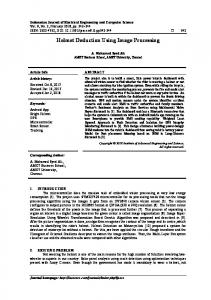
Test results showed that both GrainCheck 310 machines under–predicted the HVAC percentages by 12% to 15% when compared with the BAR results, whereas the average difference between the two GrainCheck 310 machines was only 1.54% (R2 = 0.89). On the other hand, the average difference between the original BAR inspection and the BAR re–inspection was 2.24% (R2 = 0.85) (fig. 7). Thus, it can be concluded that the consistency between the two GrainCheck 310 machines was slightly higher than that between human inspections.
98.3
89.6 83.0
70.4
60
40
20
0
HVAC 01
HVAC 02
HVAC 03
NHVAC NHVAC NHVAC NHVAC NHVAC NHVAC 01 02 03 04 05 06
FIELD SAMPLE TEST In the field sample test, model 2b was verified using sample set 3. Results from the two GrainCheck 310 machines showed a high degree of consistency, with an average difference of 0.8% between results from the two machines and an R2 of 0.81. However, both GrainCheck 310 machines under–predicted the BAR results by 15% to 16%, (R2 = 0.63 to 0.69). One possible reason for this under–prediction might be the difference in quality between the samples used to train the ANN model and the field samples used in verification. For example, the HVAC training samples used to develop model 2b were vitreous wheat kernels with high quality in color, roundness, and shape. In contrast, the HVAC field samples included many aged, dry HVAC kernels. This may have confused the ANN during classification. To improve the accuracy of HVAC classification, training samples at different quality levels should be included. The results of two GrainCheck 310 machines were also compared with the results of two manual inspections: a BAR inspection and an inspection provided by the wheat–quality extension specialists of the Department of Cereal and Food Sciences at North Dakota State University. The average difference between the two manual inspections was 1.8% (R2 = 0.75), whereas the average difference between the two machines was 0.8% (R2 = 0.81). This result once again proves that the machines tend to be more consistent than human inspectors.
Sample ID Figure 5. Classification rate of each subclass using model 2b with 100 nodes and 50 epochs.
mottled/chalky, and sprouted kernels. The classification rate for each individual subclass should, therefore, be considered when evaluating calibration models. Based on USDA GIPSA recommendations, the subclasses HVAC–02 (bleached HVAC durum kernels), NHVAC–02 (bleached NHVAC kernels), NHVAC–03 (mottled/chalky durum kernels inspected as NHVAC), and NHVAC–04 (sprouted durum kernels inspected as NHVAC) should have classification rates of greater than 85%. Model 2a approached this accuracy for the four subclasses but had low HVAC accuracy (81.9%). Several models exceeded 85% average accuracy for HVAC and NHVAC, but none exceeded 85% accuracy for HVAC–02, NHVAC–02, NHVAC–03, and NHVAC–04 while maintaining 85% or greater average HVAC and NHVAC accuracy. INSTRUMENT CONSISTENCY TEST Model 2b was used to test sample set 2 for consistency across two GrainCheck 310 machines: GC310(1) and GC310(2). Figure 6 shows the percentages of HVAC kernels in 25 samples derived from three inspections (two from the GrainCheck 310 machines and one by the BAR). To compare these inspections, two parameters were used. The first parameter (the “average error”) was defined as the mean of the differences between the HVAC percentages for each sample derived from two inspections. The second parameter is the coefficient of determination (R2) between the HVAC percentages for the 25 samples derived from two inspections.
SUMMARY AND CONCLUSIONS
The following conclusions can be drawn from this study: S An image–based grain–grading system that used ANN classifiers was used to classify durum wheat vitreousness.
100
Percentage of HVAC(%)
80 60 40 20 BAR 0
1
2
3
4
5
6
7
8
9
10 11
GC310(1) 12
13 14 15 16
17 18 19 20
GC310(2) 21 22 23 24 25
Sample ID Figure 6. Comparison of results obtained from two GrainCheck 310 machines and from the BAR examinations using sample set 2.
Vol. 46(4): 1143–1150
1149
100
Percentage of HVAC
80
60
40
20 BAR
BAR_Repicked
0 1 2
3 4 5
6 7 8
9 10 11 12 13 14 15 16 17 18 19 20 21 22 23 24 25 Sample ID
Figure 7. Comparison of results obtained from two BAR examinations using sample set 3.
S
S
S
S
S
Single–kernel images were created through pre– processing. Average hue, saturation, and intensity values for each image row and column were used as the inputs for the ANNs. Several ANN calibration models with various combinations of number of classes, number of hidden–layer nodes, and number of training epochs were developed and evaluated. Samples of three subclasses of HVAC and six subclasses of NHVAC kernels were used for model calibration and validation. Several models approached 85% to 90% correct classification for average HVAC and NHVAC. However, none of the models reached the correct classification rate of 85% (GIPSA criteria) for bleached kernels. Test results also showed that, for the 2–class and 3–class models, 50 to 100 hidden–layer nodes and 70 to 120 training epochs gave the best classification results. A 3–class model, which included a mottled class, was evaluated in order to minimize the effect of kernel orientation on detection of mottled kernels. A correction method was developed to improve the classification rates. With this correction, the classification accuracies for the mottled class and for the overall NHVAC class were improved to 91.0% and 89.4%, respectively. A 2–class calibration model was examined on two GrainCheck 310 machines to examine the transferability of the model across machines. The average difference between the classification results from the two machines was 1.5%. Field samples were examined by two GrainCheck 310 machines and two human inspectors. Test results suggested that, in order to improve the classification accuracy of the GrainCheck 310 machines, samples at different quality levels and with different ages should be used in training. Cross–examination also indicated that the machines tended to be more consistent than human inspectors. No single model provided the best classifications for all subclasses. The 2–class models may be preferred for their simplicity in calibration, but additional inputs from the GIPSA and the grain industry are needed to select the most appropriate model.
1150
REFERENCES
Delwiche, S. R, Y. Chen, and W. R. Hruschka. 1995. Differentiation of hard red wheat by near–infrared analysis of bulk samples. Cereal Chemistry 72(3): 243–247. Dexter, J. E., and B. A. Marchylo. 2000. Recent trends in durum wheat milling and pasta processing: Impact on durum wheat quality requirements. Presented at the International Workshop on Durum Wheat, Semolina, and Pasta Quality. Montpellier, France. 27 November 2000. Vienna, Austria: The International Association of Cereal Science and Technology (ICC – Europe). Dexter, J. E., P. C. Williams, N. M. Edwards, and D. G. Martin. 1988. The relationships between durum wheat vitreousness, kernel hardness, and processing quality. J. Cereal Science 7: 169–181. Dowell, F. E. 2000. Differentiating vitreous and nonvitreous durum wheat kernels by using near–infrared spectroscopy. Cereal Chemistry 77(2): 155–158. Egelberg, P., O. Mansson, and C. Peterson. 1994. Assessing cereal grain quality with a fully automated instrument using artificial neural network processing of digitized color video images. In Proc. SPIE International Symposium on Optics in Agriculture, Forestry, and Biological Processing. Boston, Mass. 2–4 November 1994. SPIE 2345: 146–158. Gonzalez, R. C., and R. E. Woods. 1992. Digital Image Processing. Boston, Mass.: Addison–Wesley. GrainCheck 310. 1999. User’s Guide. Version 3.5. Lund, Sweden: AgroVision AB. Martin, C. R., R. Rousser, and D. L. Brabec. 1993. Development of a single–kernel wheat characterization system. Trans. ASAE 36(5): 1399–1404. Sissons, M. J., B. G. Osborne, R. A. Hare, S. A. Sissons, and R. Jackson. 2000. Application of the single–kernel characterization system to durum wheat testing and quality prediction. Cereal Chemistry 77(2): 4–10. Steenhoek, L. W., M. K. Misra, C. R. Hurburgh Jr., and C. J. Bern. 2001. Implementing a computer vision system for corn kernel damage evaluation. Applied Eng. in Agric. 17(2): 235–240. Svensson, E., P. Egelberg, C. Peterson, and R. Oste. 1996. Image analysis in grain quality control. In Proc. Nordic Cereal Congress Ĉ The Nordic Cereal Industry towards Year 2000, 74–83. 12–15 May 1996. Haugesund, Norway. Nordic Cereal Association.
TRANSACTIONS OF THE ASAE