Geosci. Model Dev., 8, 1383–1394, 2015 www.geosci-model-dev.net/8/1383/2015/ doi:10.5194/gmd-8-1383-2015 © Author(s) 2015. CC Attribution 3.0 License.
Development and evaluation of the Screening Trajectory Ozone Prediction System (STOPS, version 1.0) B. H. Czader1 , P. Percell1 , D. Byun1,† , S. Kim1,* , and Y. Choi1 1 Department * currently
of Earth and Atmospheric Sciences, University of Houston, Houston, USA at: Ajou University, Suwon, South Korea
† deceased
Correspondence to: B. H. Czader (
[email protected]) Received: 10 September 2014 – Published in Geosci. Model Dev. Discuss.: 13 November 2014 Revised: 22 March 2015 – Accepted: 23 March 2015 – Published: 13 May 2015
Abstract. A hybrid Lagrangian–Eulerian based modeling tool has been developed using the Eulerian framework of the Community Multiscale Air Quality (CMAQ) model. It is a moving nest that utilizes saved original CMAQ simulation results to provide boundary conditions, initial conditions, as well as emissions and meteorological parameters necessary for a simulation. Given that these files are available, this tool can run independently of the CMAQ whole domain simulation, and it is designed to simulate source– receptor relationships upon changes in emissions. In this tool, the original CMAQ’s horizontal domain is reduced to a small sub-domain that follows a trajectory defined by the mean mixed-layer wind. It has the same vertical structure and physical and chemical interactions as CMAQ except advection calculation. The advantage of this tool compared to other Lagrangian models is its capability of utilizing realistic boundary conditions that change with space and time as well as detailed chemistry treatment. The correctness of the algorithms and the overall performance was evaluated against CMAQ simulation results. Its performance depends on the atmospheric conditions occurring during the simulation period, with the comparisons being most similar to CMAQ results under uniform wind conditions. The mean bias for surface ozone mixing ratios varies between −0.03 and −0.78 ppbV and the slope is between 0.99 and 1.01 for different analyzed cases. For complicated meteorological conditions, such as wind circulation, the simulated mixing ratios deviate from CMAQ values as a result of the Lagrangian approach of using mean wind for its movement, but are still close, with the mean bias for ozone varying between 0.07 and −4.29 ppbV and the slope varying between 0.95 and 1.06 for
different analyzed cases. For historical reasons, this hybrid Lagrangian–Eulerian based tool is named the Screening Trajectory Ozone Prediction System (STOPS), but its use is not limited to ozone prediction as, similarly to CMAQ, it can simulate concentrations of many species, including particulate matter and some toxic compounds, such as formaldehyde and 1,3-butadiene.
1
Introduction
Air pollution modeling is used to predict concentrations of pollutants and to understand physical and chemical processes involved as well as to develop necessary control strategies to improve air quality. Air pollution can be numerically simulated by several techniques that, based on the frame of reference, are generally divided into two categories: Eulerian and Lagrangian. In the Eulerian approach, the observer adopts a fixed frame of reference, which is usually the surface of the earth, with the modeling domain divided into many grid cells. This enables easy representation of pollutants’ production and transformation processes. Most Eulerian models account for atmospheric dynamics (horizontal and vertical advection and diffusion), emissions sources, and chemical production and destruction. They are often used to forecast air quality. A widely used Eulerian type model is the Community Multiscale Air Quality (CMAQ) model developed by the US Environmental Protection Agency (Byun and Schere, 2006). Lagrangian (or trajectory) models are based on species conservation equations describing atmospheric diffusion and
Published by Copernicus Publications on behalf of the European Geosciences Union.
1384
B. H. Czader et al.: Development and evaluation of the Screening Trajectory Ozone Prediction System
chemical reactions stated in terms of moving coordinates. The observer adopts moving coordinates that follow sets of hypothetical air parcels. The air parcels move along with the prevailing winds (being advected); there is no mass exchange between parcels and the surroundings except emissions of pollutants that are accounted for when the air parcels pass over source regions. Lagrangian models have much shorter run times, and are therefore more computationally efficient than their Eulerian chemical transport counterparts. However, often they do not account for chemical transformations, as the chemistry is modeled as first-order decay of pollutants; in such cases, they are unable to adequately predict the atmospheric concentrations of species with short lifetimes, such as fast-reacting ozone-forming volatile organic compounds (VOCs) and air toxins, an example of which is 1,3-butadiene. An ideal air pollution model would combine the computational efficiency of a dispersion model with the chemistry details of a chemical transport model. In other words, it would be a hybrid system merging a chemical transport model with a Lagrangian movement. This paper presents the development, validation and an example of application of a hybrid modeling approach that utilizes a Lagrangian advection scheme in an Eulerian modeling framework. This hybrid Eulerian–Lagrangian based modeling tool was designed to re-simulate only a part of a CMAQ modeling domain that is of interest. This makes it a computationally efficient tool to study a source–receptor relationship, such as the effect of emission events on the ozone concentration. In addition, it can quickly perform the analysis of physical and chemical processes, so-called process analysis, which is very time consuming to perform using the full-domain Eulerian air quality grid model. Compared to Lagrangian column models, our approach has advantages of using detailed chemistry and dynamic boundary conditions. To ensure the correctness of the algorithm’s implementation, the results were thoroughly evaluated and compared with the CMAQ simulation results. Currently, many institutions perform air quality forecasting. When implemented in the real-time air quality forecasting, this Eulerian–Lagrangian based hybrid tool can be used for a time-efficient re-simulation utilizing the same inputs as already prepared for the forecasting. As an emission source can be directly added to this tool, it can simulate effects of additional (non-routine) emission releases that are not included in the standard inventory, for example “upset” emissions from industrial facilities or wild fire emissions. Another application could be a simulation of plumes from chemical industry upon hurricane damage or upon a release of chemical or biological agents. It can also be utilized to provide detailed process analysis information (a contribution of physical and chemical processes to a simulated mixing ratio) for a moving window domain to capture chemical evolution of plumes. Since performing process analysis is very time consuming, it is not used in the air quality forecasting applications.
Geosci. Model Dev., 8, 1383–1394, 2015
A hybrid modeling approach was previously used to simulate concentrations of benzene in Houston (Stein et al., 2007). It consisted of CMAQ, the Hybrid Single Particle Lagrangian Integrated Trajectory (HYSPLIT) model, and the AMS/EPA Regulatory Model (AERMOD), where CMAQ was used to provide background concentrations. Although it successfully predicted benzene concentrations, it has limitations in AERMOD being a steady-state plume dispersion model, which does not consider chemistry and, therefore, is not suitable for simulations of more reactive species or secondary (not emitted) species. Lagrangian approaches were also developed for the purpose of detailed analysis of chemical interactions inside a plume. For example, Kimura et al. (2008) implemented algorithms that allow tracking of a plume inside the grid model (Lagrangian approach) and provided details of chemical transformations inside a plume. However, this tool does not operate independently of the host model, making re-simulation time consuming. Henderson et al. (2011) reported a pseudo-Lagrangian post-processing tool, which can be used outside the grid model to analyze its outputs in order to identify plumes and perform process analysis of the plume. In contrast, our tool can be run independently of the whole domain simulations of grid models and is designed to simulate effects upon emissions changes.
2
Development of a hybrid Eulerian–Lagrangian based modeling approach
A hybrid Eulerian–Lagrangian based modeling tool is derived from the CMAQ model in which the original CMAQ’s horizontal domain is reduced to a small sub-domain that can move along a specific trajectory (Fig. 1). Although not rigorously correct, as there is in- and out-flow through the domain boundaries that is in contrast to Lagrangian ideas, it was inspired by Lagrangian methods while taking advantage of the existing simulation machinery in CMAQ. Initially developed for ozone pollution applications, it was named the Screening Trajectory Ozone Prediction System (STOPS). Although it is not limited to ozone prediction, but similarly to CMAQ it can simulate concentrations of many species, including particulate matter and some toxic compounds, such as formaldehyde and 1,3-butadiene; for historical reasons, we continue to use the name STOPS. The CMAQ domain is divided into grid cells with a certain number of rows and columns in a horizontal direction and layers in a vertical direction. STOPS can be considered to be a sub-domain of CMAQ, which is also divided into grid cells in horizontal and vertical directions but, opposite to CMAQ, the STOPS domain moves with the mean wind as presented in Fig. 1. For each grid cell in a domain, CMAQ calculates horizontal and vertical advection, horizontal and vertical diffusion, dry and wet deposition, chemical reactions in gas, aqueous and particle phase, as well as photochemical processes and chemistry in clouds. The vertical layer strucwww.geosci-model-dev.net/8/1383/2015/
B. H. Czader et al.: Development and evaluation of the Screening Trajectory Ozone Prediction System
1385
t=tn movement of STOPS inside CMAQ domain
e u = PPBL
t=t0
1
PBL X
uL · 1σF (L)
(1)
vL · 1σF (L),
(2)
L=1 1σF (L) L=1 PBL X
e v = PPBL
1
L=1 1σF (L) L=1
where σF = 1 − σ and σ (unitless) is a scaled atmospheric pressure in a sigma coordinate system defined as follows: Inject IC and BC from CMAQ grid model
Figure 1. The conceptual model of STOPS and its movement inside the CMAQ domain.
ture and the physical and chemical processes in STOPS are the same as in the full domain CMAQ model, except that advection fluxes are obtained by utilizing the difference between a cell horizontal wind velocity and the averaged velocity of STOPS. At its starting position, the STOPS grid is aligned with the CMAQ grid, but as it moves with wind, its grid may not necessarily align with CMAQ grids (see Fig. 1). The initial location of the STOPS domain can be defined by choosing the position of the domain middle cell in terms of latitude and longitude coordinates or in terms of the column and row number in the CMAQ full domain. STOPS uses initial conditions and the dynamic boundary conditions from saved original CMAQ simulation results as well as emission and meteorological parameters as prepared for CMAQ. Because of that, STOPS movement is limited by CMAQ domain boundaries. Usually, CMAQ input and output files have hourly values. However, the calculation of science processes in CMAQ as well as in STOPS is based on a so-called synchronization time step, which is in a range of seconds to minutes and is determined by the model to satisfy the Courant condition safe advection time step. Both CMAQ and STOPS perform temporal interpolation of hourly values (initial conditions, boundary conditions, emissions, and meteorological parameters) to obtain a value at a smaller calculation time step. In STOPS, in addition to temporal interpolation, we also added spatial interpolation. It was needed for cases where the STOPS grid cells do not align with the grid cells of CMAQ input files. The trajectory for STOPS movement is calculated based on the mean wind in the middle column (hereafter mwind) that is averaged from the surface layer up to the planetary boundary layer (PBL) height and weighted by differences in pressure in each layer. The u and v components of wind (m s−1 ) were calculated according to the following equations:
www.geosci-model-dev.net/8/1383/2015/
σ=
(p − pt ) , (ps − pt )
(3)
where p is a pressure at the current level, pt is a model top pressure, and ps is a surface pressure. The trajectory can also be determined based on the averaged wind in all columns inside the STOPS domain (hereafter awind) as opposed to the trajectory based on winds in the middle column value of STOPS domain. The implementation of STOPS required modifications of the CMAQ source code, which included the following. – A Fortran-90 module, STOPS_MODLUE, was created to hold the additional data structure related to STOPS and subroutines associated with a coordinate conversion, position and velocity along the trajectory. – The SUBHFILE subroutine was modified. This subroutine determines the spatial relationship between the CMAQ grid and grids of input data; e.g., inputs with emission or meteorological data may have different horizontal domains than the CMAQ domain. The SUBHFILE subroutine was enhanced to support a moving horizontal sub-domain, whose grid points do not necessarily coincide with grid points of the input data, and which may have different locations at every synchronization time step. – The boundary subroutine, RDBCON, was modified to support a boundary thickness of three cells and to get boundary values for changing locations directly from the CMAQ full-grid concentration file. – The netCDF output file, CONC, saves only STOPS grid concentrations. In addition, an ASCII output file is generated that holds trajectory information: this is the latitude and longitude of the middle point of the STOPS domain for each output time step, along with the corresponding column and row numbers of a full CMAQ domain. – For source–receptor applications, the STOPS code was modified in a way that additional emissions can be directly injected into STOPS without the need for reprocessing an emission inventory. A name of the emitted compound(s) (in terms of model species), a location Geosci. Model Dev., 8, 1383–1394, 2015
1386
B. H. Czader et al.: Development and evaluation of the Screening Trajectory Ozone Prediction System al., 2006; Eder and Yu, 2006; Arnold and Dennis, 2006; Byun et al., 2007; Appel et al., 2012). As a moving nest, which uses the same inputs as CMAQ and utilizes CMAQ’s simulation results as dynamic boundary conditions and initial conditions, the STOPS performance is expected to be close to the results of the original CMAQ model; therefore, the code implementation was verified by comparing its simulation results with those obtained using CMAQ. The following statistical parameters were calculated for performance evaluation: Number of data set
N = NCOL · NROW · NTSTEP, 1 H¯ = N
Mean of host concentration
Figure 2. Starting locations of STOPS domains. Points indicate locations of emission point sources in Houston.
of emission release, starting and ending times, and the amount need to be specified by the user in the STOPS run script. – Given that STOPS is based on the CMAQ source code and uses the same input files, its results shall closely approximate those obtained with the 3-D CMAQ model. For the purpose of comparing STOPS results against CMAQ results, the post-processing program was developed and incorporated into the STOPS build and run scripts. With this, an additional file, HCONC, is generated from the STOPS simulations. It holds CMAQ concentrations from grid cells that correspond to the current location of STOPS. The advantage of STOPS compared to other Lagrangian models is the capability of utilizing realistic boundary conditions that change with space and time. Because of that, STOPS takes into account flow in and out of a domain, allowing for an exchange of mass between a moving domain and surroundings. This allows for simulations of conditions when a wind shear occurs for which Lagrangian models are usually not suitable. On the other hand, in the case of significant deviations in a wind speed and direction, some mass may be blown out of the STOPS simulation domain. A 1 × 1 STOPS domain is possible, but is more likely to quickly lose the effect from a perturbation in the domain, like modified emissions; thus, it is not likely to be used in practice and we did not perform tests on that domain. 3
Verification of STOPS performance
CMAQ has been found to be a reliable modeling tool whose performance has been evaluated in many studies (Smyth et Geosci. Model Dev., 8, 1383–1394, 2015
Mean of STOPS concentration
Mean bias
MB =
Mean absolute error
N X
Hi ,
(5)
i=1
N 1 X Si , S¯ = N i=1
N 1 X (Hi − Si ), N i=1
MAE =
(4)
(6)
(7)
N 1 X |Hi − Si |, N i=1
(8)
Root mean square error "
N 1 X RMSE = (Hi − Si )2 N i=1
# 12 ,
(9)
where Hi and Si correspond to instantaneous mixing ratios obtained with CMAQ and STOPS, respectively. NCOL and NROW are the numbers of STOPS columns and rows, respectively, and NTSTEP is the number of output time steps. Daily ozone maximum values from CMAQ and STOPS simulations were also calculated and are indicated as HMAX and SMAX, respectively. We performed verification for three cases: (1) a case when the STOPS domain does not move, which was performed to test an effect of boundary conditions on STOPS results; (2) cases with STOPS moving along different trajectories performed to test STOPS performance for different atmospheric conditions as well as an effect of different ways of trajectory calculation on STOPS results; and (3) cases with different STOPS domain sizes to test an effect of domain size on the STOPS results. 3.1
Effect of boundary conditions
First, the correctness of the STOPS code implementation was verified by performing STOPS simulations in the stationary mode; this is when it is not moving. In this configuration, the STOPS domain is like a CMAQ sub-domain in which the grid cells are aligned with CMAQ grid cells; thus, STOPS calculated values can be directly compared with CMAQ values from corresponding grid cells. With this setup, STOPS does not perform spatial interpolations of either initial or www.geosci-model-dev.net/8/1383/2015/
B. H. Czader et al.: Development and evaluation of the Screening Trajectory Ozone Prediction System
1387
Table 1. Specifications of STOPS domains. Name
Column and row of middle STOPS cell in a host grid
Number of padding cells in each direction
Number of STOPS domain
Number of STOPS domain
25, 30 21, 30 29, 30
10 2 2
21 5 5
21 5 5
Houston Urban Industrial
Figure 3. Comparison of CMAQ and static STOPS simulation results for 28 August for 1 h (left) and 1 min (right) output time steps. Both graphs correspond to the simulation from the Houston domain.
boundary values. The simulations were performed for three domains, differing in size and starting positions as presented in Fig. 2: the “Houston” domain, the “urban” domain that sits in the urban area and the “industrial” domain that is over the industrial region. The size of a domain is defined by the number of padding cells around the middle cell. The location of the middle column in each STOPS domain relative to the CMAQ (host) grid, the number of padding cells in each direction around the STOPS middle column, and a number of total STOPS columns and rows are presented in Table 1. Since CMAQ boundary conditions as well as other input and output files have hourly values but calculations are performed at much smaller time intervals; therefore, the boundary values are interpolated from two corresponding hourly values to match a specific computation time step. This is also the case for STOPS. For the comparison of STOPS results with CMAQ values, we used CMAQ concentrations from the grid cells corresponding to cells in the STOPS domain. These grid cells in CMAQ are not at the domain boundaries, but are inside the domain; therefore, in these grid cells, advection is calculated based on values from adjacent cells at every synchronization time step. In STOPS, these cells are at the domain boundary and hourly boundary values are interpolated for advection calculation. Because of that, we expect some differences between STOPS and CMAQ calculated mixing ratios. To justify them, CMAQ and STOPS simulations were performed for different output time steps, which were set to www.geosci-model-dev.net/8/1383/2015/
1 h, 5 min, and 1 min. This allows one to obtain CMAQ concentrations that are used as STOPS boundary conditions at small time steps, which is close to the synchronization time step, forcing CMAQ and STOPS to use the same values for advection calculation. Three sample days out of the TexAQS 2000 episode were chosen for simulations: 25, 28, and 30 August. For all cases, the STOPS simulation started at 12:00 UTC and lasted 12 h. Surface ozone values from CMAQ and STOPS were compared at each cell and each simulation’s output time step. The summary of statistical parameters calculated by CMAQ and STOPS in a stationary mode is presented in Table 2. Differences between the concentrations obtained from these two models are caused by different values at the domain boundaries. Decreasing the hourly output time step to make it closer to the synchronization time step lessens the effect of different boundary conditions as STOPS values became closer to CMAQ values. At a 1 min output time step, differences between ozone concentrations are less than 1 ppbV. Figure 3 shows a comparison of STOPS and CMAQ values from a simulation with a 1 h output time step (left) and a 1 min time step (right), with less scattering from the 1 min output time step, confirming that shortening the output time step makes STOPS results closer to CMAQ.
Geosci. Model Dev., 8, 1383–1394, 2015
1388
B. H. Czader et al.: Development and evaluation of the Screening Trajectory Ozone Prediction System
Table 2. Summary of statistical parameters for STOPS and CMAQ predicted ozone mixing ratios, when STOPS was used in the stationary mode. “hou” indicates results from the Houston domain, “ind” from the industrial domain, and “urb” from the urban domain. Name stat_hou_1h.0825 stat_hou_1h.0828 stat_hou_1h.0830 stat_hou_5m.0825 stat_hou_5m.0828 stat_hou_5m.0830 stat_hou_1m.0825 stat_hou_1m.0828 stat_hou_1m.0830 stat_ind_1h.0825 stat_ind_1h.0828 stat_ind_1h.0830 stat_ind_5m.0825 stat_ind_5m.0828 stat_ind_5m.0830 stat_ind_1m.0825 stat_ind_1m.0828 stat_ind_1m.0830 stat_urb_1h.0825 stat_urb_1h.0828 stat_urb_1h.0830 stat_urb_5m.0825 stat_urb_5m.0828 stat_urb_5m.0830 stat_urb_1m.0825 stat_urb_1m.0828 stat_urb_1m.0830
3.2
N
HMAX
SMAX
MB
MAE
RMSE
5733 5733 5733 63 945 63 945 63 945 317 961 317 961 317 961 325 325 325 3625 3625 3625 18 025 18 025 18 025 325 325 325 3625 3625 3625 18 025 18 025 18 025
162.1 115.6 158.7 166.4 116.0 160.3 166.0 115.1 158.9 108.7 88.5 145.1 111.6 88.6 148.2 112.0 86.6 146.6 162.1 69.2 145.9 165.9 70.5 145.9 165.4 69.9 144.3
162.9 115.8 158.7 167.1 115.7 160.5 166.0 115.1 158.9 113.9 88.0 147.8 112.8 87.7 148.4 112.6 86.6 146.7 161.4 70.7 148.0 167.1 71.0 146.8 165.8 69.7 144.7
−0.1894 −0.1160 −0.3089 −0.1183 0.0369 0.0167 0.0140 −0.0117 −0.0138 −0.8562 −0.7096 −1.8936 −0.5794 −0.2883 −0.4536 −0.1275 −0.0724 −0.0974 −0.9287 −0.5708 −1.5667 −0.5115 −0.2271 −0.3074 0.0214 −0.0300 −0.1970
0.3822 0.1979 0.3870 0.2067 0.1213 0.1297 0.0456 0.0365 0.0308 1.0007 0.8004 1.9774 0.6502 0.4229 0.5636 0.2107 0.1045 0.1342 1.3587 0.6402 1.5673 0.6070 0.3825 0.3411 0.2073 0.0875 0.2114
0.6820 0.3229 0.5920 0.3946 0.2075 0.2295 0.0906 0.0744 0.0715 1.4691 1.1424 2.6690 0.9494 0.6003 0.7370 0.3356 0.1426 0.2249 2.1596 0.9812 1.9527 0.9891 0.6278 0.4611 0.3132 0.1292 0.3607
Uncertainties related to movement of STOPS
a) b)
The next step in the STOPS verification was to analyze uncertainties related to the movement of a STOPS domain. A direct comparison between CMAQ and STOPS results was complicated due to the fact that, when STOPS travels with wind, its grid cells do not necessarily align with CMAQ grid cells. For the purpose of comparing STOPS values with CMAQ ones we utilized two approaches that were performed after STOPS finished its calculations. In the first approach, we aligned the STOPS grid cells with the closest CMAQ grid cells (shifted the STOPS domain) and compared the corresponding values. In the second approach, we performed spatial interpolation by calculating the weighted average from several CMAQ grid cells that overlap the STOPS grid cell. The performance evaluation was tested for these two approaches. There are two options in STOPS that can be used for a trajectory calculation. A trajectory can be determined either based on the wind in the middle column of the STOPS domain as described by Eq. (1) (mwind) or based on the averaged value from the whole STOPS domain (awind). Two smaller sub-domains shown in Fig. 2, which are urban and Geosci. Model Dev., 8, 1383–1394, 2015
August 28
August 30 August 25
Figure 4. (a) STOPS trajectories starting from the industrial subdomain. Trajectories determined based on the winds in the STOPS middle column are indicated by filled circles, and those determined based on the average winds in the whole STOPS domain with open circles. Trajectories for 25 August are indicated with red dots, those for 28 August with blue dots, and those for 30 August with green dots. Numbers next to dots show UTC time (b) details of the trajectory on 25 August.
industrial, were selected for STOPS simulations in the moving mode with the two options for trajectory calculation being tested. The days for which comparison was carried out were characterized by different meteorological conditions. 25 August 2000 was the day with complicated, circular wind patwww.geosci-model-dev.net/8/1383/2015/
B. H. Czader et al.: Development and evaluation of the Screening Trajectory Ozone Prediction System
1389
Table 3. Summary of statistical parameters for STOPS–CMAQ concentrations, when STOPS was used in the moving mode, with the starting position in the urban sub-domain. Name awind_urb_1h.0825 awind_urb_1h.0828 awind_urb_1h.0830 awind_urb_5m.0825 awind_urb_5m.0828 awind_urb_5m.0830 awind_urb_1m.0825 awind_urb_1m.0828 awind_urb_1m.0830 mwind_urb_1h.0825 mwind_urb_1h.0828 mwind_urb_1h.0830 mwind_urb_5m.0825 mwind_urb_5m.0828 mwind_urb_5m.0830 mwind_urb_1m.0825 mwind_urb_1m.0828 mwind_urb_1m.0830 awind_urb_1h_sh.0825 awind_urb_1h_sh.0828 awind_urb_1h_sh.0830 awind_urb_5m_sh.0825 awind_urb_5m_sh.0828 awind_urb_5m_sh.0830 awind_urb_1m_sh.0825 awind_urb_1m_sh.0828 awind_urb_1m_sh.0830 mwind_urb_1h_sh.0825 mwind_urb_1h_sh.0828 mwind_urb_1h_sh.0830 mwind_urb_5m_sh.0825 mwind_urb_5m_sh.0828 mwind_urb_5m_sh.0830 mwind_urb_1m_sh.0825 mwind_urb_1m_sh.0828 mwind_urb_1m_sh.0830
N
HMAX
SMAX
MB
MAE
RMSE
217 185 217 2329 1929 2329 11 545 9449 11 545 217 169 217 2329 1833 2329 11 545 9129 11 545 325 275 325 3625 3000 3625 18 025 14 750 18 025 325 250 325 3625 2850 3625 18 025 14 250 18 025
105.1 104.8 132.1 107.9 105.3 131.4 107.8 103.2 131.0 105.4 104.0 137.8 107.7 104.2 137.6 107.8 103.0 137.7 108.2 105.0 132.1 110.0 105.5 134.5 110.7 103.6 134.1 108.2 104.0 137.8 108.9 104.4 138.5 109.2 103.0 138.4
111.8 109.5 120.7 108.1 108.6 127.4 107.3 109.2 126.4 109.1 102.4 135.9 107.2 102.6 137.5 106.5 101.4 135.7 111.8 109.5 128.1 108.1 109.4 134.1 107.3 109.2 133.5 109.1 109.8 139.7 107.2 111.2 140.2 106.5 111.2 138.5
−1.7055 −0.5229 −0.6365 −0.5235 −0.062 −0.9365 −0.4557 −0.0297 −0.8205 −1.5074 −0.0594 −0.5092 −0.663 0.5222 −0.5207 −0.7221 0.6286 −0.0888 −0.4767 −0.5584 −0.1203 −0.1248 0.0152 −0.4659 0.0743 −0.0619 −0.1377 −0.1204 −0.3751 −0.1818 −0.0929 0.0849 −0.5113 −0.1237 0.1064 −0.4413
3.7246 2.4865 4.6031 2.9698 2.2454 3.9527 3.1165 2.2157 3.8026 2.6628 1.4279 3.2716 2.4906 1.8313 3.8601 2.6495 1.6039 4.1309 1.521 1.5322 2.0124 1.4191 1.3118 2.126 1.3337 1.3074 1.9516 1.7139 1.4664 2.4477 1.4659 1.1706 2.5097 1.3359 1.2086 2.4165
5.4175 4.1357 7.0249 4.1889 3.9979 5.9425 4.394 3.9464 5.743 3.8337 2.2759 5.2829 3.493 2.7969 5.7908 3.7622 2.4716 6.0413 2.3025 2.1738 3.16 2.1658 2.1861 3.1923 1.9913 2.2298 2.9423 2.5346 2.7279 3.7688 2.1744 2.0956 3.7741 1.9914 2.0841 3.5173
terns; on 28 August 2000, strong but uniform southerly winds were observed, and on 30 August, a change in winds from southeasterly to southwesterly was observed in the early afternoon hours. STOPS trajectories for these 3 days, with the starting position at the location of the industrial sub-domain, are presented in Fig. 4. Trajectories determined based on the winds in the STOPS middle column are indicated by filled circles, and those determined based on the average winds in the whole STOPS domain with open circles. All trajectories start at 12:00 UTC and end the next day at 00:00 UTC, except trajectories on 28 August that ended at 23:00 UTC due to the subdomain reaching the boundaries of the CMAQ domain earlier as an effect of strong winds on that day. On 28 and 30 August, trajectories determined by the two different methods are similar. However, as can be seen from Fig. 4b,
www.geosci-model-dev.net/8/1383/2015/
there are differences in trajectories for 25 August, especially during the first couple of hours of simulations. Both trajectories move south between 12:00 and 13:00 UTC. After that, the trajectory determined by the winds in the middle column moves east until 15:00 UTC and then west, making a circular pattern; at 17:00 UTC, it comes back to the close proximity of the starting position. On the contrary, the trajectory determined by the winds averaged in the whole STOPS domain initially moves south for a couple of hours and then continuously moves west. In order to quantify the differences between numerous options available in STOPS, several simulations were performed by changing the options one at a time. The analysis was performed for the cases when the trajectory was determined based on the winds in the middle column (mwind)
Geosci. Model Dev., 8, 1383–1394, 2015
1390
B. H. Czader et al.: Development and evaluation of the Screening Trajectory Ozone Prediction System
Table 4. Summary of statistical parameters for STOPS–CMAQ concentrations, when STOPS was used in the moving mode, with the starting position in the industrial sub-domain. Name awind_ind_1h.0825 awind_ind_1h.0828 awind_ind_1h.0830 awind_ind_5m.0825 awind_ind_5m.0828 awind_ind_5m.0830 awind_ind_1m.0825 awind_ind_1m.0828 awind_ind_1m.0830 mwind_ind_1h.0825 mwind_ind_1h.0828 mwind_ind_1h.0830 mwind_ind_5m.0825 mwind_ind_5m.0828 mwind_ind_5m.0830 mwind_ind_1m.0825 mwind_ind_1m.0828 mwind_ind_1m.0830 awind_ind_1h_sh.0825 awind_ind_1h_sh.0828 awind_ind_1h_sh.0830 awind_ind_5m_sh.0825 awind_ind_5m_sh.0828 awind_ind_5m_sh.0830 awind_ind_1m_sh.0825 awind_ind_1m_sh.0828 awind_ind_1m_sh.0830 mwind_ind_1h_sh.0825 mwind_ind_1h_sh.0828 mwind_ind_1h_sh.0830 mwind_ind_5m_sh.0825 mwind_ind_5m_sh.0828 mwind_ind_5m_sh.0830 mwind_ind_1m_sh.0825 mwind_ind_1m_sh.0828 mwind_ind_1m_sh.0830
N
HMAX
SMAX
MB
MAE
RMSE
217 201 217 2329 2281 2329 11 545 11 373 11 545 217 201 217 2329 2217 2329 11 545 11 017 11 545 325 300 325 3625 3550 3625 18 025 17 750 18 025 325 300 325 3625 3450 3625 18 025 17 200 18 025
162.1 102.0 141.4 166.2 102.0 141.7 166.0 101.5 140.4 162.1 101.6 138.0 166.4 101.7 141.8 166.0 101.1 140.0 162.1 102.6 141.5 166.4 102.4 142.4 166.0 101.9 141.0 162.1 101.9 141.1 166.4 101.7 142.4 166.0 101.2 140.8
175.6 104.5 140.1 179.9 105.4 140.5 178.6 106.2 139.7 174.0 107.3 136.8 178.7 105.6 137.4 177.7 105.7 136.6 175.6 104.5 141.3 179.9 105.4 142.2 178.6 106.2 141.1 174.0 107.3 141.3 178.7 105.6 143.1 177.7 105.7 141.6
−3.7049 −0.0743 0.5727 −4.2896 −0.0317 0.7063 −4.0882 −0.2101 0.6337 −1.2557 −0.6898 0.125 −1.0198 −0.2336 0.9498 −0.6788 −0.3779 0.743 −2.7155 −0.0949 −0.0785 −1.0475 −0.0618 −0.1354 −1.0034 −0.3176 −0.1505 −2.4646 −0.782 −0.224 −1.0628 −0.3803 −0.1763 −0.8412 −0.6202 −0.355
6.667 2.7724 2.2085 6.9033 2.8724 2.4671 7.0306 2.9622 2.3704 6.3057 2.3871 1.4439 6.3622 2.3862 2.0799 6.2981 2.2792 1.9787 4.1153 1.5528 1.6427 3.9286 1.4688 1.6548 4.0013 1.4425 1.6257 3.9385 1.5209 1.3034 4.012 1.3697 1.4963 3.9665 1.4004 1.4364
9.7334 3.6884 3.4874 10.246 3.7569 3.9274 10.1471 3.8751 3.7275 9.6064 3.4938 1.9605 9.4587 3.3116 2.8743 9.3914 3.2517 2.6921 6.5406 2.2241 2.3778 6.2411 2.0437 2.502 6.2608 2.0392 2.3916 6.1064 2.1193 1.6851 6.134 1.8761 2.0331 6.0567 1.9443 1.9099
Table 5. Statistical parameters of simulations with different STOPS domain sizes. In each case, only nine inner cells were taken for the analysis. The results correspond to the stationary case. Case 3×3 5×5 7×7 9×9 15 × 15 21 × 21
N
HMAX
SMAX
MB
MAE
RMSE
RMSE avg
117 117 117 117 117 117
162.1 162.1 162.1 162.1 162.1 162.1
158.5 161.4 159.0 160.4 160.8 162.8
−1.0496 −0.9025 −0.2914 −0.1232 0.0818 −0.0315
1.9374 1.3159 1.0090 0.6343 0.2696 0.2634
3.1827 2.1476 1.7355 1.2566 0.4597 0.4579
2.4100 1.7210 1.4075 0.9400 0.2346 0.3491
and the averaged winds in the whole STOPS domain (awind). The simulation results when the STOPS domain was shifted for the purpose of aligning its grids with CMAQ grids are
Geosci. Model Dev., 8, 1383–1394, 2015
indicated with “sh”. The naming convention used to describe each case of interest is presented in the following example: “awind_urb_1h.0825_sh” means that the trajectory was es-
www.geosci-model-dev.net/8/1383/2015/
B. H. Czader et al.: Development and evaluation of the Screening Trajectory Ozone Prediction System
1391
Figure 5. Comparison of ozone concentrations obtained with STOPS and CMAQ for 25, 28, and 30 August for the STOPS starting position in the urban sub-domain (left figures) and the industrial sub-domain (right figures). Red triangles correspond to the trajectory determined from winds in the middle column (mwind), blue crosses to the trajectory from average winds in the whole STOPS domain (awind). Compared are values from each cell in the first model layer, at every output time step. Note: the scale is adjusted to the maximum ozone concentration on a given day.
timated based on the averaged winds in the whole STOPS domain, the trajectory starting position was the urban subdomain, the model output time step was set to 1 h, the simulation was performed for 25 August, and the STOPS domain was shifted to be aligned with the host domain grid for comparison purposes. The case “awind_ urb_1h.0825” means the same as above, except that CMAQ concentrations were spatially interpolated to be compared with STOPS mixing ratios. www.geosci-model-dev.net/8/1383/2015/
Results of the statistical analysis of CMAQ and STOPS predictions of ozone concentrations when STOPS was used in the moving mode are presented in Table 3 for cases when simulations were initialized in the urban sub-domain and in Table 4 for starting positions in the industrial sub-domain.
Geosci. Model Dev., 8, 1383–1394, 2015
1392
B. H. Czader et al.: Development and evaluation of the Screening Trajectory Ozone Prediction System August 25, 2000
August 28, 2000
August 30, 2000
12 UTC
12 UTC
12 UTC
15 UTC
15 UTC
15 UTC
18 UTC
18 UTC
18 UTC
21 UTC
21 UTC
21 UTC
Figure 6. Snapshots of ozone mixing ratios as simulated by STOPS along trajectories on 25 (left), 28 (middle), and 30 August (right) when the STOPS simulation started from the industrial sub-domain. Table 6. Statistical parameters for simulations with different STOPS domain sizes, where only nine inner cells were chosen for the analysis. The results correspond to the moving case, when the trajectory starting position corresponds to the 21 and 30 CMAQ column and row, respectively. Case 3×3 5×5 7×7 9×9 15 × 15 21 × 21
N
HMAX
SMAX
MB
MAE
RMSE
RMSE avg
117 117 117 108 99 81
105.4 105.4 105.4 105.4 105.4 84.4
106.4 105.2 105.1 104.7 104.3 84.4
−0.3768 −0.2481 −0.3131 −0.4253 −0.1542 −0.3360
1.6632 1.4438 1.4116 1.2482 1.0885 1.1220
2.5934 2.2264 2.1408 1.8741 1.5237 1.7900
1.7774 1.3617 1.2725 1.0929 0.6736 0.8787
Figure 5 shows scatter plots comparing CMAQ and STOPS concentrations of ozone for 25, 28, and 30 August for the STOPS starting position in the urban sub-domain (left graphs) and industrial sub-domain (right graphs). Triangles correspond to values calculated with STOPS when its trajectory was determined based on the winds in the middle column (mwind), crosses to the trajectory obtained from the average winds in the whole STOPS domain (awind). Plotted are ozone mixing ratios from all cells in the first model layer, Geosci. Model Dev., 8, 1383–1394, 2015
at every output time step. Very good performance was found on 28 August, with the averaged mean absolute error of 1.3 and 1.5 ppbV for the urban and industrial domains, subsequently. Better agreement between CMAQ–STOPS concentration pairs was found when the STOPS trajectory was calculated based on the winds in the middle column. Shifting the STOPS domain to align it with the CMAQ grid resulted in better agreement than the case when CMAQ values had to be interpolated. www.geosci-model-dev.net/8/1383/2015/
B. H. Czader et al.: Development and evaluation of the Screening Trajectory Ozone Prediction System
1393
Table 7. As above but with different starting positions corresponding to the 25 and 30 CMAQ column and row, respectively. Case 3×3 5×5 7×7 9×9 15 × 15 21 × 21
N
HMAX
SMAX
MB
MAE
RMSE
RMSE avg
117 117 117 117 108 99
143.0 143.0 143.0 143.0 143.0 143.0
138.1 133.7 133.4 134.0 134.2 133.8
−1.1138 −0.3396 −0.1603 −0.0864 −0.0661 0.2430
3.2706 3.0431 2.9672 2.9405 3.0548 3.0527
4.9511 4.7310 4.6991 4.6791 4.8358 5.1374
3.3688 3.1896 3.2204 3.2066 3.3063 3.7556
0.05
Statistical parameters of the CMAQ–STOPS ozone mixing ratios from simulations with different domain sizes are shown in Table 5 for the stationary case and in Tables 6 and 7 for the moving cases. It can be seen that increasing the number of boundary layers around the domain of interest improves the correlation between CMAQ and stationary STOPS results. In the case of the moving mode, the simulations with bigger domains reached the boundary of the CMAQ domain earlier than the intended simulation ending time; therefore, it is not very practical.
ETHENE
O3 (ppm)
per 7560 g VOC added
HCHO
0.04
P ROP ENE B UTE1 B UTE2T
0.03
I_B UTA
0.02 0.01 0.00 6 12
7 13
8 14
9 15
10 17 11 16
12 18
13 19
14 20
15 21
16 22
17 23
18 00
Time (UTC) time (CST)
Figure 7. Changes in ozone mixing ratios due to emission spikes of different individual VOCs simulated with STOPS along the trajectory on 25 August. The values are integrated over the grid cells in the surface layer of the STOPS domain.
3.3
Effect of a domain size
Simulation results obtained with the STOPS system were validated against CMAQ calculated concentration fields for various STOPS domain sizes. The area of interest was always the same and consisted of nine inner cells in the STOPS domain. Therefore, by changing the STOPS domain size, the number of boundary layers around the area of interest differs. Six different simulations with different domain sizes of 3 × 3, 5 × 5, 7 × 7, 9 × 9, 15 × 15, and 21 × 21 cells were performed. In each case, the starting position was the same, with the middle column of the STOPS domain corresponding to the twenty-first column and thirtieth row in the CMAQ domain (urban sub-domain). Although the STOPS simulations were performed for the different domains, the final analysis was carried out based on the concentrations in the inner nine cells of the first layer. Additional analysis, based on the averaged concentration in the area of interest, was also performed. The averaging eliminates concentration differences caused by uncertainties in the horizontal transport. All simulations were carried out for 25 August 2000, for the stationary and moving modes. In the case of the moving mode, the STOPS trajectory was determined based on the wind in the middle column. For the purpose of the CMAQ–STOPS comparison, the STOPS grid was shifted to coincide with the CMAQ grid. www.geosci-model-dev.net/8/1383/2015/
4
Example of application
Here, we present an example of STOPS application for a source–receptor relationship analysis. Many industrial petrochemical and chemical manufacturing facilities are located in the Houston Ship Channel. In addition to emissions associated with regular operations, they frequently release additional, so-called “upset emissions” (Murphy and Allen, 2005). Such emission releases can dominate local emissions and result in very high ozone concentrations (Zhang et al., 2004; Nam et al., 2006). The impact of such releases can be simulated by STOPS. We performed the base case simulations as described in Czader et al. (2008) in which we used the extended version of SAPRC-99 that explicitly represents the emissions and chemistry of many individual VOCs. In addition to the base case simulation, we performed STOPS re-simulations in which an additional emission spike of several individual VOCs was added to STOPS one at the time, imitating “upset emission” release. The additional emission was added between 12:00 and 13:00 UTC at the location of the middle cell of the STOPS domain at its starting position. Figure 6 show snapshots of ozone mixing ratios in the STOPS domain on 25, 28, and 30 August 2000 along the trajectories shown in Fig. 4. The results are from the base case simulation. Figure 7 shows changes in ozone mixing ratios occurring along trajectory downwind from an emission source on 25 August that are caused by additional emissions of VOCs injected into a STOPS domain. It can be seen that different compounds affect ozone concentration to a different extent. The low reactive isobutane (I_BUTA) has a small effect on ozone, which is in contrast to trans-2-butene (BUTE2T), which, due to its Geosci. Model Dev., 8, 1383–1394, 2015
1394
B. H. Czader et al.: Development and evaluation of the Screening Trajectory Ozone Prediction System
high reactivity, has the potential to increase the ozone mixing ratio locally, close to the emission source, and with higher magnitude.
Acknowledgements. This work is dedicated to the memory of Daewon Byun (1956–2011), whose pursuit of scientific excellence as a developer of the CMAQ model continues to inspire us. Edited by: P. Jöckel
5
Summary
A hybrid Lagrangian–Eulerian based modeling tool (called STOPS) was developed as a computationally efficient 3-D grid sub-model for the purpose of evaluations of the source– receptor relationship upon release of new emissions. It is suitable for tracking a pollutant plume emitted in the morning, which then undergoes physical and chemical transformations in the well-mixed convective conditions. The correctness of its algorithms and the overall performance were evaluated against CMAQ simulation results and it was shown that STOPS is capable of predicting ozone mixing ratios in close agreement with CMAQ predictions. Its performance however depends on the trajectory calculations and the atmospheric conditions occurring during the simulation period. Better agreement between CMAQ–STOPS concentration pairs was found when the STOPS trajectory was calculated based on the winds in the middle column as compared to calculation based on the value averaged in the whole STOPS domain. Under some atmospheric conditions, such as uniform winds on 28 August, its performance was very satisfactory, with the mean bias for ozone mixing ratios varying between −0.03 and −0.78 ppbV and the slope between 0.99 and 1.01 for different analyzed cases. However, for complicated meteorological conditions, such as on 25 August, when recirculation of air occurred, its predictions deviated from CMAQ simulated values, with mean bias varying between 0.07 and −4.29 ppbV and slope varying between 0.95 and 1.06 for different analyzed cases for ozone surface mixing ratio. Averaging the surface concentration values over a STOPS domain resulted in the smaller bias between STOPS and CMAQ results. This technique is appropriate since STOPS is designed to be used for the chemical analysis rather than an analysis of individual cells in which concentration values are strongly affected by fine uncertainties in the horizontal transport. The limitation of STOPS is due to the Lagrangian movement when applied for non-uniform winds for which the plume might be dispersed outside of the STOPS domain. This is a limitation of every Lagrangian approach. The advantages of STOPS compared to Lagrangian type models are usage of realistic boundary conditions at every simulation time step as well as usage of detailed chemistry. Code availability The STOPS source code can be obtained by contacting the leading author at
[email protected].
Geosci. Model Dev., 8, 1383–1394, 2015
References Appel, K., Chemel, C., Roselle, S. J., Francis, X. V., Hu, R.-M., Sokhi, R. S., Rao, S. T., and Galmarini, S.: Examination of the Community Multiscale Air Quality (CMAQ) model performance over the North American and European domains, Atmos. Environ., 53, 142–155, 2012. Arnold, J. R. and Dennis, R. L.: Testing CMAQ chemistry sensitivities in base case and emissions control runs at SEARCH and SOS99 surface sites in the southeastern US, Atmos. Environ., 40, 5027–5040, 2006. Byun, D. and Schere, K. L.: Review of the Governing Equations, Computational Algorithms, and Other Components of the Models-3 Community Multiscale Air Quality (CMAQ) Modeling System, Appl. Mech. Rev., 59, 51–77, 2006. Byun, D. W., Kim, S.-T., and Kim, S.-B.: Evaluation of air quality models for the simulation of a high ozone episode in the Houston metropolitan area, Atmos. Environ., 41, 837–853, 2007. Czader, B. H., Byun, D. W., Kim, S.-T., and Carter, W. P. L.: A study of VOC reactivity in the Houston-Galveston air mixture utilizing an extended version of SAPRC-99 chemical mechanism, Atmos. Environ., 42, 5733–5742, 2008. Eder, B. and Yu, S.: A performance evaluation of the 2004 release of Models-3 CMAQ, Atmos. Environ., 40, 4811–4824, 2006. Henderson, B. H., Kimura, Y., McDonald-Buller, E., Allen, D. T., and Vizuete, W.: Comparison of Lagrangian process analysis tools for Eulerian air quality models, Atmos. Environ., 45, 5200– 5211, 2011. Kimura, Y., McDonald-Buller, E., Vizuete, W., and Allen, D. T.: Application of a Lagrangian process analysis tool to characterize ozone formation in Southeast Texas, Atmos. Environ., 42, 5743– 5759, 2008. Murphy, C. F. and Allen, D. T.: Hydrocarbon emissions from industrial release events in the Houston-Galveston area and their impact on ozone formation, Atmos. Environ., 39, 3785–3798, 2005. Nam, J., Kimura, Y., Vizuete, W., Murphy, C., and Allen, D. T.: Modeling the impacts of emission events on ozone formation in Houston, Texas, Atmos. Environ., 40, 5329–5341, 2006. Smyth, S. C., Jiang, W., Yin, S., Roth, H., and Giroux, E.: Evaluation of CMAQ O3 and PM2.5 performance using Pacific 2001 measurement data, Atmos. Environ., 40, 2735–2749, 2006. Stein, A. F., Isakov, V., Godowitch, J., and Draxler, R. R.: A hybrid modeling approach to resolve pollutant concentrations in an urban area, Atmos. Environ., 41, 9410–9426, 2007. Zhang, R., Lei, W., Tie, X., and Hess, P.: Industrial emissions cause extreme diurnal urban ozone variability, P. Natl. Acad. Sci. USA, 101, 6346–6350, 2004.
www.geosci-model-dev.net/8/1383/2015/