of these two systems is established by invoking the concept of similitude between the control oriented mathematical models of both turbines. Finally, preliminary ...
Development and Validation of Small-scale Model to Predict Large Wind Turbine Behavior M.Tech. Dissertation Submitted in partial fulfillment of the requirements for the degree of Master of Technology in Mechanical Engineering by Sandeep Dhar Roll No: 03310912 under the guidance of Prof. Shashikanth Suryanarayanan
DEPARTMENT OF MECHANICAL ENGINEERING INDIAN INSTITUTE OF TECHNOLOGY BOMBAY July-2006
Dissertation Approval Sheet Dissertation entitled Development and Validation of Small-scale Model to Predict Large Wind Turbine Behavior submitted by Sandeep Dhar (Roll No. 03310912) is approved for the degree of Master of Technology in Mechanical Engineering.
Examiners
..............................
..............................
Supervisor
..............................
Chairman
..............................
Date: ........................ Place: ........................
Acknowledgement This project would have never come to the current state without extensive support from a few people worth mentioning. I would like to extend my gratitude to my friend Mr. Arun K, M.Tech (TFE) for his help in undertaking the CFD analysis of S-809 wind turbine blades. I oblige much needed help from our fabricators, IMAGE MAKERS, Malad; Mr. Deepak Dangdha, JERALD ENTERPRISES, Bhandup; EL-MECH, Prabhadevi and MICROMOT CONTROLS, Bhayander. Also worth mentioning is Prof S.D. Sharma, Aerospace Dept. and Lab Assistants of High Speed Aerodynamics Lab, without whom the wind tunnel testing of turbine blades would not have taken place. Above all I would like to express my sincerest gratitude to my guide Prof. Shashikanth Suryanarayanan for his continuous much needed help in understanding various concepts used during the project, motivating me for undertaking independent research work and much needed financial help. Also my deepest regards to Prof. Shashi for helping me in making this dissertation presentable. Finally I thank Mechanical Engineering Department,IITBombay for grant of funds for the fabrication of the test-setup. Last but not the least, I would like to thank my parents and my friends for their continuous support during ups and downs of my project work and their continuous motivation to work towards betterment. Sandeep Dhar (Roll No. 03310912)
Abstract This work proposes a methodology to design a small-scale test set-up of a candidate large wind turbine. Developement of the small-scale test set-up involves design of its structural as well as its aerodynamic subsystems. Apart from the design of the subsystems, a relationship between controllers assumed for both the systems respectively, is worked out. The design of small-scale test set-up subsystems is related to the subsystems of the candidate large wind turbine through the concept of similitude. The relationship between the assumed controllers of these two systems is established by invoking the concept of similitude between the control oriented mathematical models of both turbines. Finally, preliminary power performance characterization results of the fabricated small-scale test set-up are documented.
Contents 1 Introduction
1
1.1
Problem Statement . . . . . . . . . . . . . . . . . . . . . . . . . . . . . . . .
1
1.2
Design approach . . . . . . . . . . . . . . . . . . . . . . . . . . . . . . . . .
2
1.3
Contributions of the thesis . . . . . . . . . . . . . . . . . . . . . . . . . . . .
2
1.4
Organization of the report . . . . . . . . . . . . . . . . . . . . . . . . . . . .
3
2 Preliminaries 2.1
2.2
4
Dimensional Analysis . . . . . . . . . . . . . . . . . . . . . . . . . . . . . . .
4
2.1.1
Non-Dimensional Differential Equation . . . . . . . . . . . . . . . . .
5
2.1.2
Buckhingham’s Pi theorem . . . . . . . . . . . . . . . . . . . . . . .
6
2.1.3
Criterion for similitude . . . . . . . . . . . . . . . . . . . . . . . . . .
6
2.1.4
Non-Dimensional State-Space equations . . . . . . . . . . . . . . . .
7
Wind Turbine: Preliminaries . . . . . . . . . . . . . . . . . . . . . . . . . .
8
2.2.1
Architecture Basics . . . . . . . . . . . . . . . . . . . . . . . . . . .
8
2.2.2
Power Capture Basics . . . . . . . . . . . . . . . . . . . . . . . . . .
9
2.2.3
Modeling of Horizontal-Axis Wind Turbines . . . . . . . . . . . . . .
10
2.2.4
Control Preliminaries . . . . . . . . . . . . . . . . . . . . . . . . . .
13
3 Structural Design
15
3.1
Finite Element Model . . . . . . . . . . . . . . . . . . . . . . . . . . . . . .
15
3.2
Design Considerations . . . . . . . . . . . . . . . . . . . . . . . . . . . . . .
16
3.2.1
Hub Assembly . . . . . . . . . . . . . . . . . . . . . . . . . . . . . .
16
3.2.2
Pitching Mechanism . . . . . . . . . . . . . . . . . . . . . . . . . . .
17
3.2.3
Shaft design . . . . . . . . . . . . . . . . . . . . . . . . . . . . . . . .
18
3.2.4
Generator . . . . . . . . . . . . . . . . . . . . . . . . . . . . . . . . .
18
3.2.5
Slip-Rings . . . . . . . . . . . . . . . . . . . . . . . . . . . . . . . . .
19
i
3.3
Tower . . . . . . . . . . . . . . . . . . . . . . . . . . . . . . . . . . . . . . .
4 Aerodynamic Analysis 4.1
4.2
21
Aerodynamic Similitude . . . . . . . . . . . . . . . . . . . . . . . . . . . . .
21
4.1.1
Aerodynamic Similarity approach in Wind Turbines . . . . . . . . .
22
Blade Design . . . . . . . . . . . . . . . . . . . . . . . . . . . . . . . . . . .
27
5 Similitude in Wind Turbine Controls 5.1
19
29
Control Similitude . . . . . . . . . . . . . . . . . . . . . . . . . . . . . . . .
29
5.1.1
Control Invariants . . . . . . . . . . . . . . . . . . . . . . . . . . . .
30
5.1.2
Control-Oriented Model of Candidate Large Wind Turbine . . . . .
31
5.1.3
Validation of wind turbine model . . . . . . . . . . . . . . . . . . . .
35
5.1.4
Control Invariants for Wind Turbine . . . . . . . . . . . . . . . . . .
37
6 Experimentation and Results
39
6.1
Wind tunnel testing of blades . . . . . . . . . . . . . . . . . . . . . . . . . .
39
6.2
Test-setup characterization . . . . . . . . . . . . . . . . . . . . . . . . . . .
41
6.2.1
Cp vs λ curve . . . . . . . . . . . . . . . . . . . . . . . . . . . . . . .
41
6.2.2
Losses . . . . . . . . . . . . . . . . . . . . . . . . . . . . . . . . . . .
44
7 Conclusions and Future Scope
47
7.1
Summary and Conclusions . . . . . . . . . . . . . . . . . . . . . . . . . . . .
47
7.2
Future Scope . . . . . . . . . . . . . . . . . . . . . . . . . . . . . . . . . . .
49
References
49
Appendices
51
A Derivation of Structural invariants for Wind Turbine
52
B Linearisation of Wind Turbine Model
56
C
59
Blades profile characteristics and Strucutral Drawings
D Tower, Hub, Shaft, Bearings and Blade computations
ii
64
List of Figures 2.1
(a)Horizontal axis wind turbine , (b)Wind Turbine Components
. . . . . .
8
2.2
Variation of Cp vs. λ for changing wind speed [1] . . . . . . . . . . . . . . .
9
2.3
Power curve of a Horizontal-Axis wind turbine [1] . . . . . . . . . . . . . . .
10
2.4
Wind turbine degrees of freedom [1] . . . . . . . . . . . . . . . . . . . . . .
11
2.5
Blade loading and velocity at a section XX’ . . . . . . . . . . . . . . . . . .
12
3.1
Test-setup:Hub . . . . . . . . . . . . . . . . . . . . . . . . . . . . . . . . . .
17
3.2
Motor Pitch Control Arrangement . . . . . . . . . . . . . . . . . . . . . . .
17
3.3
Shaft-Bearing arrangement . . . . . . . . . . . . . . . . . . . . . . . . . . .
18
3.4
Indirect grid connection [2] . . . . . . . . . . . . . . . . . . . . . . . . . . .
19
3.5
Slip-ring arrangement . . . . . . . . . . . . . . . . . . . . . . . . . . . . . .
19
3.6
Schematic: Test-setup Tower . . . . . . . . . . . . . . . . . . . . . . . . . .
20
4.1
Flow similarity criterion . . . . . . . . . . . . . . . . . . . . . . . . . . . . .
22
4.2
Airfoil S 809
24
4.3
(a)Velocity vs.Chord (Prototype, 2m, α = 2),(b)Velocity vs.Chord (Moedel,
. . . . . . . . . . . . . . . . . . . . . . . . . . . . . . . . . . .
150mm, α = 2, surface roughness= 0µm),(c)Velocity vs.Chord (Model, 150mm, α = 2, surface roughness= 50µm)(d)Velocity vs.Chord (Model, 150mm, α = 2, surface roughness= 300µm) . . . . . . . . . . . . . . . . . . . . . . . 4.4
25
(a)Wall shear vs.Chord (Prototype, 2m, α = 2) (b)Wall shear vs. Chord (Model, 150mm, α = 2, surface roughness= 0µm) (c)Wall shear vs. Chord (Model, 150mm, α = 2, surface roughness= 50µm) (d)Wall shear vs. Chord (Model, 150mm, α = 2, surface roughness= 300µm) . . . . . . . . . . . . . .
26
4.5
Blade Geometry . . . . . . . . . . . . . . . . . . . . . . . . . . . . . . . . .
27
4.6
(a)Max Power(watt/25mm) extracted at each section , (b)Power(watt/25mm) re-distributed to outer sections . . . . . . . . . . . . . . . . . . . . . . . . .
iii
28
5.1
Tower loading along fore-aft . . . . . . . . . . . . . . . . . . . . . . . . . . .
33
5.2
Blade Motion . . . . . . . . . . . . . . . . . . . . . . . . . . . . . . . . . . .
33
5.3
(a)Step response curves of the drive-train (b)Eigen value plot . . . . . . . .
36
6.1
(a)Wind Tunnel, (b) Blade mounting , (c) Induced surface roughness,(d) Pressure tappings on blade . . . . . . . . . . . . . . . . . . . . . . . . . . .
6.2
40
(a) Pressure along chord for varying roughness (Top) (b) Pressure along chord for varying roughness (Bottom) . . . . . . . . . . . . . . . . . . . . .
41
6.3
(a)Blower Arrangement,(b)Grid arrangement . . . . . . . . . . . . . . . . .
42
6.4
Cp Vs.λ . . . . . . . . . . . . . . . . . . . . . . . . . . . . . . . . . . . . . .
43
A.1 Shape Functions . . . . . . . . . . . . . . . . . . . . . . . . . . . . . . . . .
53
C.1 CL vs.CD [16]
. . . . . . . . . . . . . . . . . . . . . . . . . . . . . . . . . . .
59
C.2 CL CD vs.AoA[16] . . . . . . . . . . . . . . . . . . . . . . . . . . . . . . . . .
60
C.3 Root profile . . . . . . . . . . . . . . . . . . . . . . . . . . . . . . . . . . . .
60
C.4 Profile at 300mm from root . . . . . . . . . . . . . . . . . . . . . . . . . . .
60
C.5 Profile at 450mm from root . . . . . . . . . . . . . . . . . . . . . . . . . . .
61
C.6 Profile at 750mm from root . . . . . . . . . . . . . . . . . . . . . . . . . . .
61
C.7 HUB . . . . . . . . . . . . . . . . . . . . . . . . . . . . . . . . . . . . . . . .
61
C.8 Pitch . . . . . . . . . . . . . . . . . . . . . . . . . . . . . . . . . . . . . . . .
62
C.9 Blade Flange . . . . . . . . . . . . . . . . . . . . . . . . . . . . . . . . . . .
62
C.10 Motor Flange . . . . . . . . . . . . . . . . . . . . . . . . . . . . . . . . . . .
62
C.11 Tower Bearing . . . . . . . . . . . . . . . . . . . . . . . . . . . . . . . . . .
63
C.12 Gear Train . . . . . . . . . . . . . . . . . . . . . . . . . . . . . . . . . . . .
63
iv
List of Tables 6.1
Velocity Distribution . . . . . . . . . . . . . . . . . . . . . . . . . . . . . . .
43
6.2
Power output for different load resistance . . . . . . . . . . . . . . . . . . .
44
6.3
Frictional Torque observations . . . . . . . . . . . . . . . . . . . . . . . . . .
45
v
List of Symbols and Abbreviations α
Angle of attack (degrees)
β
Blade pitch angle (degrees)
φ
Blade twist (degrees)
λ
Tip-speed ratio
ω
Rotational speed (rad/s)
Ω
Rotational speed of wind turbine rotor (RPM)
π
Dimensionless number
c(r)
Chord length at radius r(mm)
k
Stiffness (N/m)
m
Mass (kg)
m0
Mass per unit length (kg/m)
ui
ith Shape function
B
Coefficient of torsional damping in bearings (Nms2 )
C
Coefficient of damping (Ns/m)
Cp
Coefficient of Power
F
External force (N)
Jeq
Equivalent mass moment of inertia (kgm2 )
K
Control gain
P
Power (watts)
Re
Reynolds number
T
Coulomb friction torque (Nm)
U∞
Free stream wind speed (m/s)
(.)b
Blade parameters/variables
(.)DT
Drive-train parameters/variables
(.)gen
Generator parameters/variables vi
(.)r
Reference parameter/variable
(.)t
Tower parameters/variables
(.∗ )
Non-dimensional parameters/variables
BEM
Blade Element Momentum
CFD
Computational Fluid Dynamics
DOF
Degrees of Freedom
FEM
Finite Element Method
LWT
Large Wind Turbine
vii
Chapter 1
Introduction The wind power industry is the fastest growing electric power industry in the world [2]. Current global installed capacity is in excess of 32000MW with a projected growth rate of 10000MW per year for the next five years. The phenomenal growth of this industry may be attributed to the rapid developments in technologies used to realize wind turbines machines used to generate electric power from the wind. For economic reasons, most of the work on wind turbine technology development has focused on large wind turbines (60-80m tower and 70-100m blade span) [2]. Though simulations provide an idea of the expected performance of a candidate large wind turbine design, turbine manufacturers perform a significant number of on-field tests on fullscale prototypes to ratify the design. On-field testing on large wind turbines proves to be expensive to most manufacturers [3, 4]. In this work, we focus on proposing a solution that reduces testing time on full-scale large, horizontal-axis prototypes. The idea is to develop a small-scale test set-up of the candidate large wind turbine design such that the experimental test results on the small-scale test setup may be used to predict the performance of the full-scale prototype. We now articulate the specific problem of interest to this thesis.
1.1
Problem Statement
Given a horizontal axis large wind turbine, subjected to a certain class of wind input, develop its geometrically scaled-down test set-up such that the behavior of the large wind turbine may be predicted from the test results of the small-scale set-up.
1
The development of the scaled-down test set-up involves the choice of right geometry and materials for its structural and the aerodynamic subsystem’s components. A simplistic approach to the problem of designing a small-scale test set-up is to geometrically scale down the dimensions of the candidate large wind turbine and establish a correlation to match the experimental results of the small-scale turbine to that of its larger counterpart. However, such an approach does not guarantee a tractable correlation between the test results on the small-scale test set-up and that on the large wind turbine. This is because, the existence of a tractable relationship between the developed forces on various turbine components, is unlikely [5].
1.2
Design approach
Our approach to the design of the small-scale set-up is to invoke the notion of similitude to arrive at decisions such as choice of material, size of components etc. The criterion for similitude is that we can find a single class of non-dimensional differential equation to which mathematical models of both the small-scale and full-scale prototypes are invertibly related. In other words, similitude is said to exist between the mathematical models of the large wind turbine and its small-scale test set-up if for each of these mathematical models there exist invertible transformations to the same non-dimensional differential equation [5] .
A few remarks are in order. • The mathematical models of the large wind turbine as well as its small-scale test setup are arrived at by treating the wind turbine as an interconnection of its structural, aerodynamic and control subsystems. • An important assumption in this analysis is that the inter-connection between the wind turbine subsystems remains the same for the candidate large wind turbine and its small-scale test set-up.
1.3
Contributions of the thesis
The contribution of this thesis are as follows:
2
• Towards the wind turbine community: We have applied concepts of similitude to the mathematical model of large wind turbine in order to establish the criterion for the design of its small-scale test set-up. To the best of our knowledge, the similitude approach has not been applied to scaled testing of large wind turbines. A similar philosophy, though, has been applied by Brennan [6] in the context of development of small-scaled vehicle-roadway system for laboratory testing of automobiles. • Towards future research at IIT Bombay: This work has led to the fabrication of a small-scale test set-up in conjunction prediction of large wind turbine performance. The test set-up would enable experimental validation of various controllers designed for a large wind turbine. Preliminary characterization of the fabricated test set-up has been done. The results of which are included in this thesis.
1.4
Organization of the report
The subsequent chapters present preliminaries and the work related to design of the smallscale test setup. Chapter 2 discusses the preliminaries of similitude and concepts involved in mathematical modeling of a large wind turbine. Chapters 3 discuss structural design of small-scale test set-up. Chapter 4 discusses issues related to aerodynamic similitude and design of small-scale-test set-up blades. Chapter 5 discusses the control related mathematical modeling of the candidate large wind turbine, validation of the mathematical model and implementation of similitude in controls. Chapter 6 lists the wind tunnel experimental results of the small-scale test set-up blades and characterisation of the test set-up. Chapter 7 lists the conclusion and future scope of this thesis.
3
Chapter 2
Preliminaries This chapter lists the necessary background required to understand the work performed. We begin with concept of dimension and its understanding from the purview of similitude analysis. Subsequently,we present a discussion on dimensionless differential equations followed by mathematical conditions for similarity between systems based on dimensionless differential equations. We further extend the concept of non-dimensionalisng to the state-space representation of linear dynamical systems. Next, we have discuss the wind turbine preliminaries- architecture of wind turbines, primary subsystems, power capture essentials and modeling approach for horizontal-axis large wind turbines.
2.1
Dimensional Analysis
Oftentimes a mechanical system’s model could be understood to be defined in a co-ordinate system whose axes are defined by [Length], [Mass] and [Time]. For example consider a spring-mass system described by the differential equation. m¨ x (t) + kx (t) = 0
(2.1)
where,’m’ and ’k’ are the parameters and ’x’ and ’t’ are the variables of the system respectively [5]. In the co-ordinate frame of [Length], [Mass] and [Time],’m’ has dimension of [Mass], ’¨ x ’ has dimension of [length] and [Time], ’k’ has dimensions of [Mass] and [Time], ’x’ has dimension of [Length]. In terms of measurable quantities (fundamental dimensions), the dimensions of variables and parameters of equation 2.1 are as follows [5, 6]: [Length]-meter(m) 4
[M ass]-kilogram(kg) [T ime]-Second(s) The variables are expressed as a numerical value accompanied by a dimension. We explain this statement through an illustration below. An expression of ’m = 1kg’ could be expressed as:
m = {1}[kg] where {1} represents the magnitude and [kg] indicates the dimensions of mass.
2.1.1
Non-Dimensional Differential Equation
Non-dimensionalising is an important process in similitude analysis. This process involves representing the parameters and variables of an expression are in terms of corresponding dimensionless parameters and variables [5]. We now illustrate the process in the context of second-order differential equation of spring-mass-damper as follows: m¨ x + cx˙ + kx = 0
(2.2)
The mass ’m’, damping coefficient ’c’, stiffness ’k’, position of mass ’x’ and time ’t’ collectively represent the physical quantities of the system [5]. The dimensions of this equation in terms of fundamental dimensions mass, length and time are kgm/s2 . We non-dimensionalise this system as follows. Define x∗ = xxr ,m∗ = mmr ,k ∗ = kkr ,t∗ = ttr , where xr ,mr ,kr ,tr , are some reference physical quantities and {x∗ , m∗ , k ∗ , t∗ } are nondimensional physical quantities. We will use {∗ } representation to a non-dimensional number or variable in the subsequent chapters. Substituting in equation 2.2 we get: � � � � 2 ∗ cr xr ∗ dx∗ mr xr ∗ d x c m + + (kr xr ) k ∗ x∗ = 0 t2r d(t∗ )2 tr dt∗ Multiplying both sides of equation 2.3 by
tr 2 mr xr
(2.3)
we get a dimensionless differential equa-
tion ∗d
m
2 x∗
dt∗ 2
� � � cr tr ∗ dx∗ kr tr 2 ∗ ∗ + + c k x =0 mr dt∗ mr �
(2.4)
The above equation represents the class of systems having the invariants (unitless numbers) equal to
cr tr mr
2
r tr and km . r
5
2.1.2
Buckhingham’s Pi theorem
The invariants derived in section 2.1.1 are some mathematical combination of certain invariants unique to a system [6, 7].The uniqueness of these specific invariants means that they are outcome of a unique mathematical combination of system parameters and variables respectively. In other words, any other mathematical combination of the system variables and parameters will lead to an invariant which may be derived from unique invariant or may not lead to any invariant at all. Buckhingham’s Pi [6, 8] gives the exact number of unique invariants associated with a system. We state the Buckingham’s Pi Theorem for the sake of completeness of our discussion Given a function of the form g(V1 , V2 , V3 , ....) = 0, WhereV1 , V2 , ..., Vn are physical quantities of system. An equivalent function of the form f (π1 , π2 , ..., πn ) = 0 can be written, where each π term is dimensionless. The number of π variables Np is given by: Np = Nv − Nd Nv is number of physical quantities and Nd is number of fundamental dimensions required to define these physical quantities.
2.1.3
Criterion for similitude
Consider two systems represented by differential equations as below: m1 x¨1 + c1 x˙1 + k1 x1 = D(x1 )
m∗
d2 x∗ dt∗ 2
m2 x¨2 + c2 x˙2 + k2 x2 = D(x2 ) � � � � kr tr 2 ∗ ∗ cr tr ∗ dx∗ + c k x = D0 (x∗ ) + mr dt∗ mr
(2.5) (2.6) (2.7)
Let Equation 2.7 be a dimensionless differential equation, where ’D’, ’D0 ’ are differential operators. Systems described by Equations 2.5 and 2.6 are said to be similar if there exist invertible transformations T1 and T2 that takes both these systems to Equation 2.7. In 6
other words, the necessary and sufficient condition of similitude between two systems is that the mathematical models of one be related by a bijective transformation to that of the other [5].
2.1.4
Non-Dimensional State-Space equations
We now apply the above definition of similitude for linear systems represented in state-space form. The standard state-space representation of a linear time invariant system is: x(t) ˙ = Ax(t) + Bu(t) y(t) = Cx(t) + Du(t)
(2.8)
The procedure for non-dimensionalising the above system has been illustrated by Brennen [6, 7, 9]. It has been shown that the resulting non-dimensional state-space equation is of the form. {x} ˙ = [A]{x} + [B]{u} {y} = [C]{x} + [D]{u} where {x} = [X] {x∗ },{u} = [U ] {u∗ },{y} = [N ] {y ∗ } and t = St∗ , also {x} ˙ =
(2.9) d([X]{x∗ }) . dSt∗
The matrices [X],[U]and[N] are diagonal matrices with elements along principal diagonal having dimensions same as elements of {x}, {u} and {y} respectively [9]. Substituting in Equation 2.9, we get
[X] ˙∗ {x } = [A][X]{x∗ } + [B][U ]{u∗ } S [N ] {y ∗ } = [C][X]{x∗ } + [D][U ]{u∗ }
(2.10)
Simplifying the above equation, we get {x˙∗ } = S[X]−1 [A][X]{x∗ } + S[X]−1 [B][U ]{u∗ } {y ∗ } = [N ]−1 [C][X]{x∗ } + [N ]−1 [D][U ]{u∗ }
(2.11)
The generalised form of non-dimensional state-space equation may be written as: {x˙∗ } = [A]∗ {x∗ } + [B]∗ {u∗ } {y ∗ } = [C]∗ {x∗ } + [D]∗ {u∗ } Comparing coefficients of Equation 2.11 and Equation 2.12, we have 7
(2.12)
(a)
(b)
Figure 2.1: (a)Horizontal axis wind turbine , (b)Wind Turbine Components [A]∗ = S[X]−1 [A][X] [B]∗ = S[X]−1 [B][U ] [C]∗ = [N ]−1 [C][X] [D]∗ = [N ]−1 [D][U ]
2.2 2.2.1
Wind Turbine: Preliminaries Architecture Basics
The architecture of the class of wind turbine considered in this report is as follows. It consists of a three bladed rotor Fig 2.1(a), which partially converts wind energy to its rotational energy through aerodynamic interaction between wind and its blades. This rotational energy is fed into a generator usually through a step-up gear box. We will consider the wind turbine as being composed of the following interconnected subsystems: structural, aerodynamic and control. The structural subsystem consists of the blades, the shaft-gear box arrangement (Fig 2.1 (b)), termed as the drive-train, and the tower. The aerodynamic subsystem captures the interaction between the wind and the blades. The control subsystem includes the generator, pitching arrangement and their associated controllers [3]. The pitching arrangement is housed within the hub of the rotor and provides the capability to rotate the blades about their axes.
8
2.2.2
Power Capture Basics
We now present elementary information on the power capture characteristics of horizontalasix wind turbines. Consider a steady, homogeneous, incompressible and inviscid wind field with an average free stream velocity of U∞ incident upon a horizontal-axis wind turbine with rotor area A. The kinetic energy passing through the rotor area in unit time may be computed as: P= 12 ρAU∞ 3 where ρ is the air density. The ratio of mechanical power, Pmech , captured by the turbine rotor to the available power P is defined as Coefficient-of-Power, Cp . i.e., Cp = Pmech P Betz showed that under steady, homogeneous, incompressible and inviscid flow conditions [3], the maximum achievable Cp is
16 27 .
It is well-known that the coefficient-of-power Cp varies with the tip speed ratio(λ),which is ratio of the tangential velocity of the rotating blade tip to the free-stream wind velocity. Fig. 2.2 shows a typical Cp −λ curve for a wind turbine. As can be seen from this figure, the maximum power capture efficiency is realized at particular value of λ, say (λopt ) - termed as the optimal tip-speed ratio.
Figure 2.2: Variation of Cp vs. λ for changing wind speed [1]
9
Fig 2.3 shows the typical ”Power Curve” of a horizontal-axis large wind turbine. The small wind speed at which the power capture become possible is termed as cut-in speed (Vcut−in ). With the increase in the wind speed, the power output of the wind turbine also increases. As the wind speed reaches the rated wind speed (Vrated ), the wind turbine delivers the rated power. For any further increase in wind speed above Vrated , the wind turbine power capture is limited to the rated power till the wind speed reaches cut-out speed (Vcut−out ). After the cut-out speed, the wind turbine is shut-down to avoid any structural failure.
Figure 2.3: Power curve of a Horizontal-Axis wind turbine [1]
2.2.3
Modeling of Horizontal-Axis Wind Turbines
Structural Model Different approaches are used to model the structural subsystems. The choice of a particular approach is dictated by what the model would be used for. If high-fidelity models are required, the components of structural subsystem are often modeled as distributed parameter systems with infinite degrees of freedom. However, such model often turn out to be computationally expensive to deal with. A more popular approach is to treat the turbine as an interconnection of elements with only a finite number of degrees of freedom (DOF). This approach to modeling is used in a host of simulators such as FAST [10]. For example, the turbine may be treated as a system with the following degrees of freedom [1] (see Fig 2.4).
10
Figure 2.4: Wind turbine degrees of freedom [1] • In and out of the plane (of rotor plane) DOF of blades termed as blade-edge and blade flap motions respectively. • Fore-aft and side-to-side motion of the tower. • Torsional DOF of the drive train. One such finite-degree of freedom formulation to describe the motion of the structural elements is the Finite Element formulation (FEM) [11] wherein the dominant modes of the distributed parameter system are considered [12]. The equations of motion under this formulation take the following form: [M ]{¨ x} + [C]{x} ˙ + [k]{x} = {F }
(2.13)
where, [M] is the mass matrix, [C] is the damping matrix, [k] is the stiffness matrix of the associate with the structural system, [F] is the force matrix and {x} is the nodal displacements.
The mass and stiffness matrices may be worked out as shown below [13]: Z 0 ui uj dx mij = m0
(2.14)
l
where mij
Z 0 1 x2 dui duj d2 ui d2 uj 2 2 dx + (1 − m Ω l ) dx (2.15) kij = EI 0 2 2 2 l2 dx dx l l dx dx represents the i − j th element of the mass matrix [M], ui , uj are the assumed Z
0
mode shape functions, kij is the i − j th element of the stiffness matrix, Ω is rotational speed of the rotor, EI is the structural rigidity, ’l’ is the length of the structural component and m0 is the linear density of the structural component.
11
Aerodynamic Model We use the Blade Element Momentum theory (BEM) [3] to arrive at the mathematical representation of the blade-wind interaction. We wish to mention that there are other methods of representing blade-wind interaction such as Vortex Wake methods, Acceleration Potential method[3]. Our choice of the BEM method is motivated by the simplicity of constructions used in the BEM theory.
The basic assumption of BEM theory is that the force on a blade element is solely due to change of momentum of air which passes through the annulus swept by the blade element. Due to the airfoil shape of the blade cross-section, lift ’L’ and drag ’D’ forces are produced over the blade. These forces may be computed as follows: L = CL 12 ρAW 2 D = CD 21 ρAW 2 where CL and CD are coefficients of lift and drag respectively,’A’ is the blade cross-section, ’W’ is the relative speed at entry of the blade section and ’ρ’ is the density of medium. It is observed that CL and CD are dependent on the angle between the relative wind velocity ’W’ and chord ’c’. This angle is also called as angle of attack (AoA), represented by α in this thesis. The sum total of the vector combination of these forces is responsible for producing rotating torque as well as the thrust on the blades as shown in Fig 2.5. It should
Figure 2.5: Blade loading and velocity at a section XX’ be noted that the BEM model neglects fluid-structure interaction.
12
2.2.4
Control Preliminaries
Control-Oriented Modeling Control-oriented modeling is the process of arriving at a mathematical description of the dynamics of wind turbines which lends itself amenable to the use of established control design tools. In the absence of any control law, such a model is said to represent openloop dynamics of the wind turbine. Oftentimes, control-oriented models are arrived at by linearizing the dynamical equations about chosen operating points. Consider the system of equations described in Eqn. 2.13. Linearizing this system about a chosen operating point (x0 , F0 ), we get: [M ]{∆¨ x} + [C]{∆x} ˙ + [k]{∆x} = {∆F }
(2.16)
where [∆F] and {∆x} are small variations in force matrix and the nodal displacement matrix considered about the chosen operating point. We therefore rearrange Equation 2.16 as below {∆¨ x} = −[M ]−1 [C]{∆x} ˙ + [M ]−1 [k]{∆x} + [M ]−1 {∆F }
∆x˙
zeros{n, n}
= ∆xvel ˙ [M ]−1 [k]
zeros{n, m} + −[M ]−1 [C] ∆xvel [M ]−1 [∆F ] I{n, n}
∆x
(2.17)
(2.18)
where ’{∆x}’ is the positional states matrix, ’{∆xvel }’ is the time derivative of positional states matrix, ’zeros{n, n}’ is n × n zero matrix and ’I’ is an identity matrix for the wind turbine system having ’n’ degrees of freedom and ’m’ control inputs. Equation 2.18 also represents the wind turbine system’s state-space representation. Hence, the system dynamics matrix [A] and the input dynamics matrix [B] of the wind turbine system are as below.
[A] =
zeros{n, n}
I{n, n}
−[M ]−1 [k]
−[M ]−1 [C]
[B] =
zeros{n, m} −[M ]−1 [∆F ]
Full-State feedback controller A feedback controller computes the control inputs to be applied to the process under control based on measured real-time information. For example, in case of wind turbines the feed13
back controller computes the control inputs for generator torque control applications based on the measured values of generator rotational speed. Such a controller when expressed mathematically alongwith the control-oriented model of the process, represent closed-loop dynamics of the process. The structure of feedback controllers can be varied. We now introduce the reader to the full-state feedback control structure. Consider a linear, time-invariant model in state-space form: x(t) ˙ = Ax(t) + Bu(t) y(t) = Cx(t) + Du(t)
(2.19)
where, ’x(t)’ represents the state variable, ’x(t)’ ˙ is time derivative of the state variable, ’A’ represents the relationship between x(t)and x(t) ˙ in absence of any control input, ’u(t)’ is the control variable, ’B’ represents the effect of control variable on the system dynamics, ’y(t)’ is output variable of interest of the system, ’C’ relates output variable to the state variable and ’D’ represents the effect of control variable on the output variable of the system. We term the control law as a full-state feedback law if u(t) is chosen so that u(t) = Kx(t). Such a control law assumes that every state variable is measured.
14
Chapter 3
Structural Design This chapter discusses the application of the concept of similitude to the problem of design of structural components of small-scale test set-up. The output of the design process is to arrive at decisions regarding the materials and the dimensions of the small-scale test set-up’s structural components. We begin with mathematical modeling of the structural subsystem from which we derive non-dimensional parameters that characterize the structural dynamics. The structural components of the test set-up are designed so that the non-dimensional parameters associated with the structural models of the small scale set-up and the large wind turbine remain invariant.
3.1
Finite Element Model
We use a finite degree of freedom mathematical model to describe the structural dynamics (see Chapter 2). Specifically, we model the structure as an interconnection of elements with the following degrees of freedom: • The flap-wise DOF for all three blades. • The fore-aft DOF for the tower. • The number of degrees of freedom for each of the blades and the tower are three viz. the DOF of base, the DOF of the mid-point and the DOF of the tip of the blades and the tower respectively.
15
We have used Finite Element Method [11] (see Chapter 2) to arrive at the mathematical models of the structural componenets viz. the blades, the drive-train and the tower. The interconnections between component models are dictated by constraints imposed by the horizontal-axis structure of the class of wind turbines of interest to this work [3].
3.2
Design Considerations
The concept of similitude is invoked to arrive at the structural invariants which form the basis for designing the small-scale test set-up. Details of this process are included in Appendix A. The parameters and variables of the candidate large wind turbine and its test set-up are related through these structural invariants which are listed below: •
m0 tlt m0 blb represents
•
Et It lb 3 Eb Ib lt 3
•
1 represents Ω2 tb 2
•
Eb Ib represents lb 3 m0 bΩb 2
the ratio of mass of tower to mass of blade.
represents the ratio of tower stiffness to blade stiffness. the angle made by the blade at any given time instant. the ratio of the blade natural frequency to blade rotational fre-
quency. We have used these invariants to estimate the dimensions of the strutural components of the test set-up. However, in some cases we have had to use considerations not dictated by similtude conditions such as load bearing ability to arrive at the final dimensions of the component in question. Computations associated with checking load bearing ability are included in Appendix D. We now detail the considerations in the design of various structural components.
3.2.1
Hub Assembly
The hub assembly provides space for housing blade pitch drives. The following issues were considered during the design of the hub assembly. • Ease of location of blades accurately around the hub. • Dynamic balance of hub. • Ease in manufacturing.
16
Figure 3.1: Test-setup:Hub • Placement of pitch-control motor. The triangular hub arrangement addresses the issue of accurate placement of blades at equal angles (120o apart) with respect to each other. The dimensions of the hub of the small-scale test set-up were governed by the dimensions of pitch-control motor and ease in replacing the motor whenever required. Detailed design computations for the hub are given in Appendix D. Fig 3.1 shows a schematic of the hub.
3.2.2
Pitching Mechanism
Figure 3.2: Motor Pitch Control Arrangement As mentioned earlier, the pitching mechanism is used to rotate the blades about their axes (pitching). This mechanism is mounted in the hub housing and consists of feedback controlled motors as well as a gear-train. Pitching action is usually active in above-rated wind speed (see Chapter 2) conditions [3] to regulate power capture. Apart from regulation of power, a large positive pitch angle through the pitching mechanism enables a large starting torque for the wind turbine rotor. 17
The pitching arrangement for the small-scale test set-up is shown in Figure 3.2. The motor used in this case is a permanent magnet DC motor. A reduction ratio of ’2’ is used from the motor to the blade flange. The choice of the reduction ratio was dictated by the maximum desired pitching rate consideration (≈ 10 rad/s). We have used two bearings between the blade mounting flange and motor flange to provide improved support (Fig 3.2). Pitch Motor Selection The pitch motors are selected based on considerations of expected aerodynamic twisting moment [14] on the blade. The twisting moment is due to asymmetry in the airfoil shape. The desired torque capacity of the pitch motor and its gearing ratio are determined based on blade inertia, expected friction and the specification for desired maximum pitching rate. Indicative computations related to motor selection are given in Appendix D.
3.2.3
Shaft design
Figure 3.3: Shaft-Bearing arrangement The drive shaft has been designed based on the consideration of drive-train similitude (Appendix A). The design was checked for structural safety under aerodynamic torsion and in bending due to weight of hub-assembly. We have assumed a limiting value 3mm of allowable deflection to determine the length shaft between the support bearings (Appendix D).
3.2.4
Generator
Wind turbine generators are unusual compared to other generating units attached to the electrical grid. One reason is that the generator has to provide desired torque demands over a wide range of rotor speeds. Large wind turbines use doubly-fed induction generators for variable speed operation. Such machines allow generator torque demand to be controlled independent of generator speed/slip [3]. In doing so, variable frequency AC output is generated. 18
Figure 3.4: Indirect grid connection [2] The cost of rectifying the variable frequency output from an AC generator to a constant frequency output to the grid is high. This has led to the selection of separately excited DC generator. Another advantage in using separate excitation in generator is the ease of realization of a variable generator torque demand with/without change of field flux [3]. The DC generator parameter selection was based on expected arodynamic power, expected rotational speed of rotor and medium of dissipation of generated electric power. Details of selection are given in Appendix D
3.2.5
Slip-Rings
Slip-rings provide a mechanism to transmit signals from a rotating member such as the hub-assembly to a stationary member such as a control terminal. In our case, the pitchmotor actuation signals along with transmission of encoder signal from each pitching unit needs to be transmitted to/from the controller. To accommodate for the terminals of each
Figure 3.5: Slip-ring arrangement motor and terminals of encoder, 21 brass rings of carrying capacity of 2.3A( maximum pitch motor current), have been fabricated as shown in Fig 3.5 above.
3.3
Tower
The hub-assembly alongwith the drive shaft and generator are mounted on the tower. The type of towers prevelant in wind turbine industry are lattice towers and tubular towers [2]. 19
The tubular design was selected for the small-scale test set-up based on considerations of structural strength and ease of fabrication. The design procedure involved maintaining equivalence between the following dimensionless numbers associated with the candidate m0 tlt large wind turbine as well as the test set-up: ( m and 0 blb
Et It lb 3 ). Eb Ib lt 3
The resulting design
was checked for the possibility of faliure under aerodynamic loads and buckling loads. Appendix D details the associated computations.
Figure 3.6: Schematic: Test-setup Tower
20
Chapter 4
Aerodynamic Analysis The dynamics of wind turbines are dictated, significantly, by wind-blade interaction. The preservation of the qualitative nature of the wind-blade interaction between the candidate large wind turbine and the small-scale test set-up ensures aerodynamic simialrity. To preserve the nature of this interaction, we need to study the factors influencing wind-blade interaction. This chapter discusses the study of the factors influencing wind-blade interaction. The results of this study have been used to design the blades of the small-scale test set-up. The blade design process involves arriving at aerodynamically appropriate geometry of the blade and selection of the airfoil profile.
4.1
Aerodynamic Similitude
An aerodynamic system consists of the dynamics of fluid surface interaction. Aerodynamic similarity between any two aerodynamic systems, consisting of fluid-surface interaction, is ensured if • The surfaces of both the aerodynamic systems are geometrically similar [15] (see Fig 4.1). • Assuming the two geometrically similar aerodynamic surfaces are in separate/same flow field, the angle-of-attack with respective free stream velocities is same. • Assuming the two geometrically similar aerodynamic surfaces are in separate/same flow field, the ratio between the forces and moments over their respective surfaces is constant. This condition is also termed as dynamic similarity. 21
The geometric similarity between two aerodynamic surfaces is achieved by ensuring constant geometric scaling factor between the surfaces. In other words, all the geometrical dimensions of one of the surface should scale by the same factor to arrive at the dimensions of other surface. The dynamic similarity between the geometrically similar aerodynamic systems is ensured through similarity of flow. By similarity of flow, we understand: • The point of transition from laminar to turbulence in flow over the two geometrically similar aerodynamic surfaces, is also geometrically similarly located (see Fig 4.1). • The Reynolds number (Re), an indicative of aerodynamic forces, should be equal across the flow over the two geometrically similar aerodynamic surfaces.
Figure 4.1: Flow similarity criterion Remark: It is known that the lift and drag forces in a flow over an aerodynamic surface are functions of Re and the angle-of-attack [15] between the free stream velocity and the surface. The blades of the candidate large wind turbine and the test set-up are assumed to be in same flow-medium (air) and at same AoA with the medium’s free stream velocity. We now discuss the aerodynamic similarity approach applied to the design of the blade of small-scale test set-up.
4.1.1
Aerodynamic Similarity approach in Wind Turbines
The small-scale test set-up blade has been designed by applying aerodynamic similarity to the candidate large wind turbine blade. In this context, following has been done. • The candidate large wind turbine blade is geometrically scaled down to arrive at the 22
dimensions of the the small-scale test set-up blades. Same airfoil shape has been used for both the blades. • Flow similarity, between these blades is ensured by locating the transition point geometrically similar between the blades. • Equality of Reynolds number, for the flow over both the aerodynamic surfaces has been attempted by varying the surface roughness of the test set-up blades. It is well-known that local Reynolds number is a function of local velocity of the flow [15]. Apart from that, magnitude of Reynolds number also indicates to the laminar/turbulent condition in a flow. Hence, the change in surface roughness of an aerodynamic surface affects the local Reynolds number by changing the local velocities of flow. This change may lead to desired flow conditions over the portion(s) of interest on the aerodynamic surface. We have used Computational fluid dynamics (CFD) simulation package FLUENT to investigate aerodynamic similarity between the blades of the candidate large wind turbine and the test set-up. CFD Analysis The results from the CFD analysis of the candiate large wind turbine blade have been used to locate of the transition point of the flow for the small-scale test set-up. Further, we have analysed the test set-up blades in FLUENT, for various surface roughnesses. The results of this analysis have been used to decide upon a roughness that ensures flow similarity between the blades. Some of the important considerations during the analysis have been as follows: • We have used 2-D airfoil sections of both the blades, considered at the root, for the CFD analysis. • The flow medium (air) and the free stream velocity is assumed to be same for both of the blades. • The effects of blade rotation, such as cross-flow, are neglected while analysis of both the blades. The airfoil used is S-809 [16] shown in Fig 4.2 : Airfoil Characteristics are listed below: • Maximum thickness = 0.2099 c 23
Figure 4.2: Airfoil S 809 • Camber = 0.0095 c • Lead edge radius = 0.0123 c • Trailing edge angle (degrees) = 3.68 where ’c’ is the chord length of the blade. As indicated earlier in this chapter, the flow conditions as well as the forces associated with the flow are jointly indicated by the Reynolds number of the flow. Apart from the Reynolds number, Wall shear stress - shear stress due to interaction of fluid elements with the surface of the aerodynamic body, also indicates to the flow condition over an aerodynamic surface [15]. Hence, we have plotted the variation of local velocity - indicator to local ’Re’ and local wall shear stress for the candidate large wind turbine blade and the test set-up blade (see Fig 4.3 and Fig 4.4). Analysis of the plots, Fig 4.3(a) and Fig4.4(a), of the candidate wind turbine blade, indicates to the drag value (ratio of wall shear stress to dynamic head) of 0.011 at local Reynolds number of 280000, at the point located at a distance of 150mm from the entry point the blade. This flow condition over the candidate wind turbine blade corresponds to turbulence on Drag vs. Re line plotted by Liepmann and Dhawan [15] using flow theories of Blasius and Prandlt [15]. Hence, knowing the transition point and the pattern of flow in the candidate wind turbine blade, following was attempted of the geometrically similar test set-up blade. • Locating the transition point geometrically similarly (3mm from the entry point) on the test set-up blade. • In order to make local ’Re’ same between the candidate wind turbine and the test set-up, the surface roughness of the test set-up blade was varied from 0 µm-300 µm.
24
(a)
(b)
(c)
(d)
Figure 4.3: (a)Velocity vs.Chord (Prototype, 2m, α = 2),(b)Velocity vs.Chord (Moedel, 150mm, α = 2, surface roughness= 0µm),(c)Velocity vs.Chord (Model, 150mm, α = 2, surface roughness= 50µm)(d)Velocity vs.Chord (Model, 150mm, α = 2, surface roughness= 300µm)
25
(a)
(b)
(c)
(d)
Figure 4.4: (a)Wall shear vs.Chord (Prototype, 2m, α = 2) (b)Wall shear vs. Chord (Model, 150mm, α = 2, surface roughness= 0µm) (c)Wall shear vs. Chord (Model, 150mm, α = 2, surface roughness= 50µm) (d)Wall shear vs. Chord (Model, 150mm, α = 2, surface roughness= 300µm) This change of surface roughness in was brought into effect for the portions after the transition point of the small-scale test set-up. The CFD analysis of the test set-up blades revealed following results. Fig 4.3 (b),(c)and (d) represents the velocity profile and Fig 4.4 (b),(c)and (d) represent wall-shear stress over the test set-up blade. The magnitudes of local drag and corresponding local Reynolds number in each test cases indicated to the laminar flow over the test set-up blade on Liepmann-Dhawan line . A possible approach to overcome this situation is mechanically making the flow turbulent at the transition point of the test set-up blade. This approach is commonly employed in experimental aerodynamics [17]. 26
We now discuss the methodology involved with the test set-up blade design.
4.2
Blade Design
Small-scale test set-up blade design involves computing the pitch angle ’β’ and airfoil selection for various cross-sections (Fig. 4.5) of the blade from root to tip. Pitch angle is defined as the angle between the chord of a cross-section with the plane of rotation of the blade (Fig 2.5). Two separate blade designs have been attempted for the blade of the small-scale test set-up. The blade design that indicated to increased aerodynamic power out of the possible test set-up blade was used in test set-up blade fabrication.
Figure 4.5: Blade Geometry We list the assumptions for blade design as follows: • Geometrically similar airfoils have been assumed for all the cross-sections of the blade. • The variation of flow velocity at inlet of the blade, along the length of the blade, is neglected. • The test set-up blade length has been computed by geometrically scaling the length of the candidate large wind turbine blade. • Sections of 25mm each have been considered along the radial distance, from the bladeroot to the blade-tip. The initial design of the small-scale test set-up blade was based on maximum power capture at all cross-sections [3]. Accordingly the desired value of lift at all the cross-sections was computed. Variation of chord of blade sections was assumed to vary linearly from root to tip. Using this design technique, the power curve obtained is shown in Fig 4.6(a). However, 27
Power/25mm section
Power/25mm section
35
45 40
30
Power(watt)
Power (watt)
35 25
20
15
30 25 20 15
10
5 0
10
100
200
300 400 500 Blade−length(mm)
600
5 0
700
(a)
100
200
300 400 500 Blade−length(mm)
600
700
(b)
Figure 4.6: (a)Max Power(watt/25mm) extracted at each section , (b)Power(watt/25mm) re-distributed to outer sections the total aerodynamic power output computed for this design was much less than expected power(Appendix D). Therefore another design was attempted as follows. It is known that the outer part of blade is active in power capture than root portion. Hence, another test set-up blade design based on redistribution of power captured, by increasing the chord length in outer portions of the blade, was undertaken. In this case, the design computations were worked out by assuming coefficient of lift of the blade to be constant throughout the blade length. The chord length was assumed to remain constant from root to 1/3 of blade length. Further the chord length is assumed to change linearly till the blade tip (Fig 4.5). It is observed that implementing the maximum power captured in outer section of blade leads to higher aerodynamic power output (Fig4.6(b))compared to the earlier design. Details of the blade design computation are given in Appendix D. Material used in blades has been Fiber Reinforced Plastic, commonly used in large wind turbine fabrication. The material exhibits excellent toughness to large centrifugal force yet is lighter than other candidate materials.
28
Chapter 5
Similitude in Wind Turbine Controls In this chapter, we discuss the procedure used to find the invariants that relate the controllers of the candidate large wind turbine and the small-scale test set-up. The procedure has been worked out, in general, for linear time-invariant similar systems by nondimensionalising their control-oriented models. A reduced degree of freedom control-oriented model for the candidate large wind turbine has been constructed. We have applied the procedure to the control-oriented mathematical model of the candidate large wind turbine and symbolically determined the control related invariants. We will assume that the controllers themselves are linear and time-invariant.
5.1
Control Similitude
Control similitude is said to exist between two closed-loop systems if: • The control-oriented mathematical models representing the open-loop dynamics of the controlled processes are similar (see Chapter 2). • There exist invertible maps from each of the controllers to a single non-dimensional differential equation. The non-dimensional parameters of such a non-dimensional differential equation will be termed as control invariants.
29
5.1.1
Control Invariants
In this section, we arrive at a condition for the existence of a single non-dimensional differential equation to which two controllers map invertibly. We will assume that the controlled processes are described by linear time-invariant control-oriented models. Further, we will assume that the controllers have a state-feedback structure (see Chapter 2). Consider a linear, time-invariant model of a controlled process described as follows: {x} ˙ = [A]{x} + [B]{u} {y} = [C]{x} + [D]{u}
(5.1)
Under the influence of a state-feedback control law, the governing dynamics are defined by: {x} ˙ = [A]{x} − [B][K]{x}
(5.2)
Using the procedure described in Chapter 2, we non-dimnesionalize Equation 5.2 to get: {x˙∗ } = S[X]−1 ([A] − [B][K])[X]{x∗ }
(5.3)
where S and [X] are as defined in Chapter 2. Again as discussed in Chapter 2 , the non-dimensional form of Equations 5.2 may be expressed as: {x˙∗ } = [A]∗ {x∗ } + [B]∗ {u∗ } {y ∗ } = [C]∗ {x∗ } + [D]∗ {u∗ }
(5.4)
where [A∗ ], [B ∗ ],[C ∗ ] and [D∗ ] are non-dimensional state matrices(see Chapter 2). Suppose Equation 5.4 are subject to a non-dimensional state-feedback law as shown below. {u∗ } = −[K ∗ ]{x∗ } Then the governing dynamics of the non-dimensional differential equation (Equation 5.4) becomes: {x˙∗ } = [A∗ ]{x∗ } − [B ∗ ][K ∗ ]{x∗ }
(5.5)
Comparing coefficients of Equation 5.3 and Equation 5.5, we have: [B ∗ ][K ∗ ] = S[X]−1 [B][K][X] 30
(5.6)
We know [B ∗ ] = S[X]−1 [B][U ] from Chapter2, substituting in Equation 5.6, we get [B][U ][K ∗ ] = [B][K][X]
(5.7)
where [K ∗ ] is the non-dimensional control gain matrix and its elements are the control invariants. [K ∗ ] can explicitly written as follows [K ∗ ] = [U ]−1 [K][X]
(5.8)
If [B]T [B] exists and is invertible for both the systems. Thus we have established a procedure to compute the control invariants associated with the non-dimensional law given the dimensional form of a state-feedback controller. The inverse procedure will be used to compute the gains of the state-feedback controller for a class of systems whose open-loop models are similar. We now work out a control-oriented mathematical model of the candidate large wind turbine. This model will be used for the synthesis of a controller for the large wind turbine. Subsequently, the result shown above will be invoked to determine the controller for the small scale test set-up.
5.1.2
Control-Oriented Model of Candidate Large Wind Turbine
The definition of a control-oriented mathematical model has been explained in Chapter 2. In this section, we discuss the methodology to arrive at such a model for the candidate large wind turbine. We represent the dynamics of the subsystems of the candidate large wind turbine by second-order differential equations. The mathematical expressions for the associated disturbance inputs (undesired inputs) and the control inputs (desired inputs) have been worked out. The mathematical combination of the differential equations and these input expressions represent the control-oriented mathematical model of the candidate large wind turbine. The mathematical model of the candidate large wind turbine exhibits an inherent nonlinearity. This non-linear mathematical model has been linearised about rated wind speed. The subsystem components modeled, are the blades, the tower, the drive-train and the generator. Assumptions to control-oriented mathematical modeling of the candidate large wind turbine, are as below: • Flap-wise degree of freedom of the blades and fore-aft degree of freedom of the tower are considered in the modeling process. 31
• Each blade is considered as a separate component in the modeling process. • The components of structural subsystem are assumed to be single degree of freedom lumped-mass systems. • The chosen operating point for linearisation [18] is at the rated wind speed. • The dynamics of generator and the drive-train do not effect tower as well as blade dynamics along their assumed DOF (Gyroscopic couple neglected). The controlling inputs considered are the blade pitch angle and generator torque demand. The disturbance input in each of the component’s mathematical model is the aerodynamic force due to wind transmitted on each of the components. We now discuss the mathematical modeling of the components of as follows: Notations used Some of the notations while modeling of the large wind turbine are as follows: {m, C, k, x, l}t refer to parameters of tower, {m, C, k, x, l}bi refer to the parameters of blades and ’i’ refers to the blade number, ρ is wind density and cb is large wind turbine blade root chord length, Ω is blade rotational speed and U∞ is the free stream wind speed. ’a’ is axial induction factor [3] and a ´ refers to tangential flow factor [3]. φ is blade twist angle(sum of AoA and blade pitch angle). {C, k, J, θ}DT refers to drive-train parameters. {C, J}gen refers to generator parameters.
Tower dynamics Tower dynamics along fore-aft DOF are influenced by aerodynamic forces, transmitted through blades, as a result of blade-wind interaction [3]. The inertial forces and damping reaction from blade flap-wise vibrations also contribute to the tower dynamics. While modeling, the tower mass is considered lumped at the tower-top, as shown in Fig5.1. Hence, we have mathematical model of the tower as: mt x¨t + Ct x˙t + kt xt = −mb1 x¨b1 − Cb1 x˙b1 − mb2 x¨b2 − Cb2 x˙b2 − mb3 x¨b3 − Cb3 x˙b3 � � �� 3 + ρcb U∞ 2 lb 1 − a2 + Ω2 lb 2 1 + a ´2 [CL cos φ − CD sin φ] 2 32
(5.9)
Figure 5.1: Tower loading along fore-aft Blade dynamics Though all the blades are represented by separate equations in the final model, we assume the basic structure of these equations to be same. Hence a generalised blade mathematical model is worked out. The dynamics of blade along flap-wise DOF are affected by the change in momentum of air flowing over it(BEM, Chapter 2). The acceleration of blade’s inertial frame of reference, assumed to be located at the tower top, induces additional inertial forces on the blade along the assumed DOF. The blade mass is assumed to be lumped at the tip of the blade. Hence, the mathematical model of blade is as follows:
Figure 5.2: Blade Motion
mbi x¨bi + Cbi x˙bi + kbi xbi = −mbi x¨t − Cbi x˙t � � �� 1 + ρcb U∞ 2 lb 1 − a2 + Ω2 lb 2 1 + a ´2 [CL cos φ − CD sin φ] 2 33
(5.10)
where i = 1,2,3 denotes the blade number.
Drive-train torsion Drive-train experiences the torsion due to the torque produced by vector combination of lift and drag forces over the candidate wind turbine blades(Chapter2). The orientation of blades as shown in Fig 5.2 also creates a component of blade inertial and damping force along the plane of rotation. Such an orientation of the blades results in an additional torque induced on the drive-train. The equivalent rotational inertia consisting of the rotor, the generator and the shaft is considered at an extremity of the drive-train. Hence the drive-train mathematical model is as follows: ¨ + CDT θ˙bi + kDT θDT = Jeq θDT " � U∞ 2 lb 2 1 − a2 3 + ρcb + 2 2
3 X
i=1 Ω2 lb 4
(−mbi lb i sin φx¨bi − Cbi sin φx˙bi ) 1+a ´2 4
�#
[CL sin φ − CD cos φ]
(5.11)
Generator Generator free-body motion (generator rotation) is the outcome of the aerodynamic torque transmitted through drive-train and the variable torque demand across the generator armature [3] on the generator inertia. The dynamics of drive-train influences free-body motion of the generator inertia by inducing fluctuations in the transmitted aerodynamic torque. These fluctuations are the result of drive-train inherent flexibility and the aerodynamic torque transmitted to it through the rotor. Thus the mathematical model of generator is as follows: (Jgen + Jrot ) Ω˙ + Cgen Ω =
3 X
(−mbi lb i sin φx¨bi − Cbi sin φx˙bi )
i=1
"
U∞ 2 l b 2 3 + ρcb 2 2
� 1 − a2
+
Ω2 lb 4
−Jg enθD¨T − Cg enθD˙ T # � 1+a ´2 [CL sin φ − CD cos φ] 4
(5.12)
The equations of the candidate large wind turbine components above are non-linear due to non-linear mathematical expressions of aerodynamic forces and moments. The equations of the candidate large wind turbine are linearised about rated wind speed. These linearised equations are represented in state-space prior to validation and non-dimensionalising. Lin-
34
earisation and subsequent conversion to state-space representation, of the candidate large wind turbine model is given in Appendix B.
5.1.3
Validation of wind turbine model
The validation of the linearised candidate large wind turbine model is important to ascertain the results obtained after non-dimensionalising the model. The validation of our linearsied mathematical model requires corroboration of its dynamics with previously known dynamics of the candidate large wind turbine. We have validated our linearised mathematical model against the results of the wind turbine simulator FAST, developed by 1 NREL-USA.
FAST [10] has an in built linearisation routine to compute an operating point to linearise their in-built non-linear model of the wind turbine about that point. FAST undertakes multi-point linearisation where in, along the wind turbine azimuth, multiple operating points are selected. The in-built wind turbine non-linear model of FAST is linearised at each of the selected operating points. Finally, an azimuth averaged model is computed by averaging the system matrices ([A], [B], [C], [D]) obtained at these points. Computation of average system matrices of the candidate large wind turbine in FAST has been undertaken using inbuilt routines of FAST. MATLAB as a tool has been used to compare the stepresponse of both the models (Fig 5.3). Fig 5.3(a) shows the plot of step-response curves for the drive-train dynamics of FASTlinearsied model and our version of the candidate large wind turbine model. It is observed that the step-response curve of our version of the wind turbine model and that of FAST differ in magnitude across same time history. However, the nature of the curves remains similar across the two systems. Apart from the step-response curves, we have plotted eigen values of state matrices of both the systems ([A]). The magnitude as well as the sign (+/-) of an eigen value dictates the nature and evolution of the input-response curves of a system. Fig 5.3(b) shows the eigen value plots for both the systems. Except for the eigen values of drive-train dynamics, all other eigen values observe a close match between the systems. The eigen-values of drivetrain dynamics are located on left-most side of eigen value plot(see Fig 5.3(b)) for both the systems. 1
NREL-USA- National Renewable Energy Lab, USA
35
Pole−Zero Map
200
FAST Linearised Model
150
Step Response
0.14 FAST Linearised Model
100
0.12
50 Imaginary Axis
Amplitude
0.1
0.08
−50
0.06
−100
0.04
−150
0.02
0 0
0
10
20
30
40
50
60
70
80
90
100
−200 −25
−20
−15
−10
−5
Real Axis
Time (sec)
(a)
(b)
Figure 5.3: (a)Step response curves of the drive-train (b)Eigen value plot The difference in drive-train step-response curve indicate to relatively larger value to stiffness in our version of drive-train mathematical model. This difference is also observed between the eigen values of drive-train dynamics for both the models Some of the reasons for the observed anomalies may be as follows: • Modeling of aerodynamic forces and moments in our mathematical model may differ from that of FAST-linearised model. • Limitations in our complete knowledge of wind turbine structural-aerodynamic interaction such as the effect of aero-elasticity on the structural components, specially blades. • Single DOF lumped-mass representation of structural subsystem components, specially drive-train. A possible solution to the observed anomalies is the use of lumped-mass representation of structural components with multi-degree of freedom. Multi DOF control-oriented large wind turbine model based on assumed modes method, considering all possible DOF of the wind turbine system, has been worked out and verified by Dixit [1]. Due to time limitations, we have not been able to include a such an approach and verify its results. We now work out the symbolic representation of control invariants for the class of wind 36
0
turbines considered.
5.1.4
Control Invariants for Wind Turbine
The symbolic representation of control invariants is worked out by symbolically non- dimensionalising assumed state feedback controller of the candidate large wind turbine. In the process, we assume that the symbolic representation of the invariants remains unaffected by the choice of the control-oriented mathematical model used. Hence, the controller gains for candidate large wind turbine controller are as below: Kφ1 Kφ2 Kφ3 Kφ4 Kφ5 Kphi6 Kφ7 Kφ8 Kφ9 Kφ10 Kφ11 Kφ12 [K] = Kt1 Kt2 Kt3 Kt4 Kt5 Kt6 Kt7 Kt8 Kt9 Kt10 Kt11 Kt12 where Kφi and Kti (i = 1 − 12) symbolically represent the assumed pitch controller gains and generator torque controller gains (Appendix B). We use Equation 5.7 to arrive at the non-dimensional gain matrix as follows. According to Equation 5.7 [K ∗ ] = [U ]−1 [K][X]
(5.13)
We have define [U]and [X] matrices(Chapter2) as:
[U ] =
1
0
0 Pt
where ’Pt ’ is the desired power corresponding to the required generator torque at some λopt . � � (d) = lt ; 1; 1; lb ; lb ; lb ; kCt ltt ; Ω; Ω; kCb lbb ; kCb lbb ; kCb lbb
[X] =diag(d,0)
Hence, the non dimensional gain matrix according to Equation 5.13 after replacing the [U], [K] and [X] in the equation is
2 4
[K ∗ ] = Kφ1 lt
Kφ2
kφ3
Kφ4 lb
Kφ5 lb
Kphi6 lb
Kφ7 kt lt Ct
Kt1 lt Pt
Kt2 Pt
Kt3 Pt
Kt4 lb Pt
Kt5 lb Pt
Kt6 lb Pt
Kt7 kt lt Pt Ct
37
Kφ8 Ω
Kφ9 Ω
Kφ10 kb lb Cb
Kφ11 kb lb Cb
Kφ12 kb lb Cb
Kt8 Ω Pt
Kt9 Ω Pt
Kt10 kb lb Pt Cb
Kt11 kb lb Pt Cb
Kt12 kb lb Pt Cb
3 5
The [B]T [B] matrix for the candidate large wind turbine mathematical model has been symbolically verified as invertible using MATLAB. We thus claim, that the elements of [K ∗ ] above are the control invariants between the candidate wind turbine and the small-scale test set-up.
38
Chapter 6
Experimentation and Results In order to experimentally verify the CFD analysis (Chapter4) of blades and characterise the fabricated test set-up, following set of experiments have been performed. • Wind tunnel testing of small-scale test set-up blades for their aerodynamic characteristics and verification of CFD analysis results. • Testing of fabricated test-setup in artificially created wind field to determine the Cp vs.λ characteristics. • Characterisation of dynamic losses for the test set-up. This chapter lists the experimental procedure and the associated results of the experimentation performed on the fabricated test-set-up. We start with the details of the wind tunnel testing of the fabricated blades of the test set-up.
6.1
Wind tunnel testing of blades
The scope of CFD analysis is limited by the limitations imposed by mathematical representation of various fluid flow phenomenon such as wake dynamics [3]. In the absence of a tractable mathematical expressions for such dynamics, their effects are not seen in CFD simulations. This situation calls for experimental validation of CFD simulation predictions through wind tunnel testing of the test set-up blades. The small-scale test set-up blade has been tested in a closed-jet wind tunnel [17] (see Fig 6.1(a)) with conduit cross-section of 500mm × 500mm. A careful attempt has been made to experimentally capture the flow conditions assumed for CFD analysis (Chapter 4). 39
(a)
(b)
(c)
(d)
Figure 6.1: (a)Wind Tunnel, (b) Blade mounting , (c) Induced surface roughness,(d) Pressure tappings on blade In order to take readings for the local pressure across the blade surface, pressure taps have been inserted at appropriate distances from the leading edge (see Fig 6.1(d)). The location of the pressure taps was decided based on CFD predicted flow characteristics over the test set-up blade. The tappings were connected through pipes, as shown in Fig 6.1(b), to the digital manometer for pressure readings. To emulate different surface roughness, different grades (220, 150, 120, 80, 60) of flint paper have been used. The portion of the test set-up blade to which the surface roughness was induced was dictated by known location (CFD analysis) of the transition point on the blade (refer Chapter 4). Fig 6.2 (a) and (b) shows the plot of pressure over an airfoil section of the test setup for changing surface roughness. It is observed that for various surface roughnesses used, there is no sudden change in pressure variation over the test set-up blade. This apparently indicates to the laminar flow over the test set-up blade. The confirmation of the transition point may be explicitly infered from the velocity of the points close to the blade surface. The measurement of velocities at points close to the blade surface involves extensive instrumentation and careful observation. Due to time and resource limitations,
40
(a)
(b)
Figure 6.2: (a) Pressure along chord for varying roughness (Top) (b) Pressure along chord for varying roughness (Bottom) we could not undertake the experimentaion.
6.2 6.2.1
Test-setup characterization Cp vs λ curve
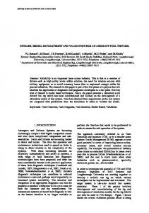
Power performance characterization of the fabricated test set-up is necessary before other experiments are performed on it. Specifically, we obtain the Cp vs λ, the basic characteristic curve associated with the test set-up (see Chapter 2).
An artificially created the wind
field is used for this purpose. The artificial wind-field has been created using industrial fans arranged as shown in Figure 6.3(a) in front of the test-setup. In order to estimate aerodynamic efficiency of test set-up blades, we need to compute the kinetic energy passing through the rotor plane in unit time. This quantity is a function of average flow flow velocity. Since it was observed that the velocity of flow across the artificial wind-field is non-uniform, velocity measurements were taken over the entire rotor plane at various grid points (Figure 6.3 (b)) tabulated in Table 6.1. We use the cubic mean of measured velocity at these grid points to compute the mean velocity of the wind field as follows. Vavg =
�
V11 3 + V12 3 + .... + V66 3 18
� 13
(6.1)
This aerodynamic power is converted into mechanical power (Pmech ) through wind-blade
41
(a)
(b)
Figure 6.3: (a)Blower Arrangement,(b)Grid arrangement interaction and fed to the DC generator through the drive shaft. The DC generator converts the available mechanical power to the electrical power (Pelec. ). It may be noted that the output power of a generator depends on the armature current and rotational speed. The terminal/output voltage of a generator is given by: Ea = ka φa ωg
(6.2)
where Ea is generator terminal voltage,ka is the generator torque constant,φa is field flux assumed constant (see Chapter 3)and ωg is generator rotational speed (rad/s). It is well known that generator armature develops an opposing torque to the input shaft torque, an effect of Lorentz forces [19]. Thus as the current in the armature increases, the generator torque demand [3] to the wind turbine rotor also increases. Hence increasing the load resistance increases the generator rotational speed. We now give the expression for the generator output power. Assuming no induction losses in the generator, the electrical power in the generator is given by: Pelec. = Ea IL = ka φa ωg IL
(6.3)
where IL is the current across the load resistor. It is straightforward to see that maximum aerodynamic/electric power captured (assuming constant losses), for a given wind speed and fixed pitch angle will be when (ωg IL ) is maximized. In order to determine electrical power output across the DC generator armature a variable resistive load is used across the armature. The resistive load is varied using a rheostat in order to compute maximum electric power. The observations are listed in Table 6.2. It is observed that the maximum 42
Table 6.1: Velocity Distribution Grid Line no.
Angle
Velocities (1-3) on grid lines (m/s)
1
0
2.6
5.2
1.5
2
60
5.1
4.6
5.3
3
120
5.7
7.4
5.4
4
180
4.7
5.6
1.6
5
240
0.9
7.0
1.4
6
300
2.8
7.0
0.3
Vavg = 4.94 m/s Paerodynamic =194 watts
electric power is extracted at 186 RPM for λ = 3.89 (
ω( rotor)Rrotor ). Vavg
This value of λ is the
optimum tip-speed ratio of the test set-up for the artificial wind field’s averaged speed. The variation electric power with λ, for the artificial wind field’s averaged speed, is shown in Fig6.4. We now details the experimentation process involved in loss characterisation of the fabricated test set-up. Cp vs tip speed ratio at Vavg=4.94m/s
0.028 0.026 0.024 0.022
Cp
0.02 0.018 0.016 0.014 0.012 0.01 0.008 3
3.5
4 Tip−speed ratio
Figure 6.4: Cp Vs.λ
43
4.5
Table 6.2: Power output for different load resistance
6.2.2
Ωg
Load Current
Load Resistance
Power
λ
145
0.95
5
4.51
3.03
154
0.8
7
4.48
3.22
177
0.71
10
5.041
3.7
186
0.66
12
5.2272
3.89
193
0.58
15
5.046
4.04
200
0.47
20
4.418
4.19
210
0.37
25
3.4225
4.39
214
0.32
30
3.072
4.48
223
0.2
40
1.6
4.67
Losses
In order to estimate the input mechanical power to the DC generator for computing aerodynamic efficiency, we need to estimate the losses in the test set-up. These losses take the form of viscous losses in the bearings and the contact frictional losses in the slip-rings. The viscous losses are often characterized by the coefficient of viscous friction and the contact losses by coloumb friction. The coulomb friction and viscous friction for the set-up are estimated by free-running the test set-up rotor-generator assembly upto certain rotational speed and then allowed to come to rest. The inertial rotational kinetic energy of the assembly is dissipated through the viscous and coloumb frictional torque. Assuming uniform retardation, we can compute the frictional torque as follows: J
dω + Bω + T = 0 dt
(6.4)
Where J-mass moment of inertia of rotor and generator combines, B-viscous friction coefficient, T-coulomb friction torque and ω-rotor rotational speed (rad/s). We can rearrange
44
Equation 6.4 as: J
dω = −Bω − T dt
(6.5)
We have used following difference form of the above equation. J
∆ω = −Bωavg − T ∆t
(6.6)
For a small time interval we assume linear decrease in speed. Hence T and B could be found out by solving Equation 6.6 for any two set of observations listed in Table 6.3. Table 6.3: Frictional Torque observations Ωi
Time
Angular acceleration
Ωavg
B
T
110
35
-
-
-
-
100
33.33
-0.62
11
-
-
90
32
-
-
-
-
80
30
-0.524
8.9
0.25
.89
70
26
-
-
-
-
60
21
-0.21
6.8
-
-
PF ric = 50.53 watts
From the values of B and F computed using Equation 6.6 and observations listed in Table 6.3, the frictional power loss (PF ric ) at the rotational speed of 186RPM was computed. In the process of measurement of the generators efficiency at 186 RPM, the generator was rotated at this speed using a DC motor with maximum power load (12 ohms)across its armature (see Table 7.2). From the measurements of input electric power (Vin , Iin ) to the DC motor and its known core losses, the input mechanical power to the generator shaft was computed. Similar measurements for generator electric power were made. Thus the efficiency of the generator at 186 RPM was computed to be ≈40 percent. As mentioned earlier, the rotational speed of 186 RPM also corresponds to maximum aerodynamic power captured by the test set-up blades for the average artificial wind speed. Therefore the aerodynamic efficiency of the blades at λoptimum = 3.89 for Vavg =4.94m/s may be computed as below:
45
Pmechanicalat186 =
Pelectricalat186 0.4
+ PF ric
therefore Pmechanicalat186 ≈ 64watts Hence the aerodynamic efficiency of the test set-up is Pmechanicalat186 Paerodynamic
≈
64 194
46
≈ 33percent
Chapter 7
Conclusions and Future Scope 7.1
Summary and Conclusions
The aim of this thesis work was to develop a scaled-down version of a large wind turbine so that the large wind turbine’s performance could be predicted from the results on the scale down version. The methodology proposed in the thesis in this regards has been shown to be an outcome of application of similitude to the associated subsystems of the large wind turbine whose scaled-down version is desired. We now summarize the work undertaken in this thesis regarding the development of the scaled-down version of a candidate large wind turbine. • Structural: We formulated Finite Element model of the candidate large wind turbine. This model was non-dimensionalised to arrive at structural invariants which were used to design the structural components of the small-scale test set-up. • Aerodynamic: The conditions under which the blades of the candidate large wind turbine and that of the test set-up tend to be aerodynamically similar were studied and established using a CFD package. The results of the study were used to design the blades of the small-scale test-set-up. • Controls: The procedure to compute control invariants between similar control processes was established. A control-oriented mathematical model for the candidate large wind 47
turbine with reduced DOF was worked out and validated with the results from FAST. A symbolic representation of the state-feedback controller for this model was used to arrive at control invariants between the candidate wind turbine and the test-setup. • Characterisation: Wind tunnel testing of the fabricated test-setup blade was performed to verify the results obtained during CFD analysis. The fabricated small-scale test set-up was characterised by plotting Cp -λ curve and loss computations for the test set-up. The results of the test set-up characterisation were also used to determine the aerodynamic efficiency of the blades of the set-up. The following conclusions were drawn: • The dynamics of structural subsystems of a candidate large wind turbine and its small-scale version are said to be similar if they are described by identical structural invariants. The design of the structural subsystem of the small-scale wind turbine utilizes this notion of similarity in conjunction with the structural safety considerations. • If surface roughness of blade may be chosen as a free parameter, then the flow pattern over geometrically similar candidate large wind turbine and its small-scale test set-up blades can be maintained similar. Such a situation will ensure aerodynamic similarity between the candidate large wind turbine and its small-scale test set-up. • The non-dimensional controller to which the controllers of similar systems may be invertibly mapped exists, if the product of their input dynamics matrix and its transpose is invertible. • Single degree of freedom lumped-mass representation of large wind turbine’s drivetrain dynamics leads to analytically simple but structurally stiff system. However such a representation of drive-train dynamics does not capture its structural behavior accurately. • Aerodynamic power captured by the small-scale test set-up, maximizes at λ = 3.89 for the artificial wind speed of 4.94 m/s. This value of tip-speed ratio of the test set-up is the optimum tip-speed ratio for the wind speed of 4.94m/s.
48
7.2
Future Scope
This thesis has not addressed several problems related to the small-scale test set-up. Some of these problem of immediate interest are listed below: • Complete validation of the designed small-scale test set-up. This may be done by corroborating the test results on the test set-up, obtained under same external conditions as that of the candidate large wind turbine, with some known performance results of the candidate wind turbine. • Experimental verification of the CFD analysis including the effects of blade rotation. This may be undertaken using valid experimental procedure to measure local flow velocities over the test set-up blade. The local flow velocities indicate to the local Reynolds number over the flow. • Defining the performance limit of a class of large wind turbines. This may be achieved by representing the performance limit models non-dimensionally. • Verification of the proposed control invariants between the candidate large wind turbine and the small-scale test set-up. This may be achieved by designing a statefeedback controller for one of the wind turbines and estimating the state feedback gains for other system using proposed control invariants. The performance results may be simulated for control-oriented models of both the turbines and compared for verification.
49
References [1] A.Dixit. Developement of LTI/LTV Model Templated for Control of Large Wind Turbines. Master Degree Thesis, IIT Bombay, India, 2005. [2] http://www.windpower.org. [3] N.Jenkins T.Burton, D.Sharpe and E.Bossanyi. Wind Energy Handbook. John Wiley Sons Ltd., New York, USA, 2001. [4] ASME/ANSI PTC 42-1988. Wind Turbines: Perofrmance test codes. The American Society of Mechanical Engineers, New York,USA, 1988. [5] E.Szucs.
Similitude and Modeling.
Elsevier Scientific Publishing Company, New
York,USA, 1980. [6] S.Brennan. On Size and Control The use of Dimensional Analysis in Controller Design. Ph.D. Thesis, UIUC-Urbana, Illinois USA, 2002. [7] S.Brennan. Similarity Conditions for Comparing Closed-Loop Vehicle Roll and Pitch Dynamics. Proceedings of the American Control Conference, pp.3393-3398, 2004. [8] E.Buckingham. On Physically Similar Syatems: Illustrations of the use of dimensional equations. Physical Review, vol.4, pp.345-376, 1914. [9] A.Alleyne S.Brennan. H-infinity Vehicle Control Using NonDimensional Perturbation Measures. Proceedings of the American Control Conference, pp.2534-2539, 2002. [10] M.L.Buhl Jr. J.M.Jonkman. FAST User’s Guide: Technical Report. National Renewable Energy Lab, Colorado USA, 2004. [11] J.N.Reddy. Finite Element Methods. McGraw-Hill Inc., Princeton NJ,USA, 1993.
50
[12] W.T.Thompson. Theory of Vibration with Application. CBS Publishers and Distributors, New Delhi India, 1988. [13] L.Meirovitch. Analytical Methods in Vibration. The McMillan Company,, CollierMcMillan Ltd., London, 1967. [14] A.Pope. Basic Wing and Aiffoil Theory. McGraw Hill Book Company Inc., New York, USA, 1951. [15] H.Shlichting. Boundary Layer Theory. McGraw Hill Book Company Inc., New York, USA, 1960. [16] http://turbulence.kmip.net/doc/Science/FluidMech. [17] A.K.Martynov. Practial Aerodynamics. Pergamon Press, New York USA, 1965. [18] K.Ogata. Modern Control Engineering. Prentice-Hall of India, New Delhi India, 2005. [19] P.C.Sen. Principles of Electrical Machines and Power Electronics. John Wiley Sons, New York,USA, 1997.
51
Appendix A
Derivation of Structural invariants for Wind Turbine In general the FEM equation of a structure under no load in matrix form may be as below: [M ] {¨ x} + [C] {x} ˙ + [k] {x} = 0
(A-1)
In present discussion, the damping has been neglected. The component wise calculation of mass and stiffness matrix is undertaken using Galerkin’s method [11] with shape function [11] being the quadratic shape functions (Fig. A.1), written as follows. Assuming W as local displacement of blade/ tower structure along its length, W may be defined as: W = u 1 q1 + u 2 q2 + u 3 q3
(A-2)
where 3x l
u1 = 1 −
+
2x2 l2
+
4x2 l2
u3 = − xl +
2x2 l2
u2 =
4x l
And ui are the shape functions and qi are the node point displacements. We have formulated the FEM model considering only one of the three blades and the tower. The formulation is carried out with the assumption that remaining blades interact with the tower in similar fashion. External forces are neglected in the formulation. The mass and stiffness matrix elements may be worked out from equations below: Z 0 ui uj dx (A-3) mij = m l
52
Figure A.1: Shape Functions
kij = EI
Z
0 l
1 d2 ui d2 uj 2 2 2 2 dx + 2 mΩ l dx dx
where ui,j are ith − j th shape functions.
Z
l
0
(1 −
x2 dui duj ) dx l2 dx dx
(A-4)
It may be seen that the stiffness formula (kij ) involves the term for centrifugal stiffness in blades, which absent in tower. Thus the procedure for FEM model formulation for the wind turbine is as follows: • First, the component level (blade/tower/drive-train) FEM formulation is worked out for the the wind turbine structural subsystem • Next, the component level FEM equations are combined according to the interconnection between the components. • Finally, the boundary/external conditions [11] are applied at the assumed nodes of the structural subsystem to get the FEM equation for the structural subsystem. We now directly give the FEM formulation for the blades and the tower as below. Blade equation
2 15
mb lb 49 15
−1 30
49 15 8 15 1 15
� 16 −32 16 q˙1 � E I b b 1 + −32 64 −32 q˙2 15 q¨2 lb3 2 q˙3 16 −32 16 q¨3 15 31 −32 −1 0 15 q1 15 15 2 32 8 −1 = +mb Ωb lb 15 0 5 6 q2 1 −1 2 q3 0 15 6 5
−1 30 q¨1
for the tower, the equation is:
53
(A-5)
0 q˙ � � 1 E I t t 1 + −32 64 −32 q˙2 = 0 3 15 q¨2 lt 2 0 q ¨ q˙3 16 −32 16 3 15
49 15
2 15
(mt lt ) 49 15
8 15
−1 30
−1 30 q¨1
1 15
16
−32
16
(A-6)
Combining Equation A-5 and Equation A-6 following their interconnectivity, we get: Mass matrix as:
2mt lt 15
49mt lt 15
−1mt lt 30
49mt lt 15
8mt lt 15
1mt lt 15
0
0
49mb lb 15 8mb lb 15 1mb lb 15
−1mb lb 30 1mb lb 15 2mb lb 15
0
0
−1mt lt 30
1mT lt 15
0
0
0
0
2 15 {mt lt + mb lb } 49mb lb 15 −1mb lb 30
16Et It lt3
−32Et It lt3
−16Et It lt3
0
0
−32Et It lt3
64Et It lt3
−32Et It lt3
0
0
16Et It lt3
−32Et It lt3
−32Eb Ib lb3
−16Eb Ib lb3
0
0
−32Eb Ib lb3
64Eb Ib lb3
−32Eb Ib lb3
0
0
16Eb Ib lb3
−32Eb Ib lb3
−16Eb Ib lb3
Stiffness matrix as
16{ Elt3It + t
Eb Ib } lb3
Centrifugal stiffness matrix can be modified as:
0 0
0
0
0
0 0 0 0 0 −32 1 mb Ω2 lb 0 0 31 15 15 15 8 −1 0 0 −32 15 5 6 1 −1 2 0 0 15 6 5 Now for similarity all the elements of the mass and stiffness matrix are to be non-dimensionalised (see Chapter 2). Element (3,3) of mass and stiffness matrices need to be analyzed first since it representd the common node for the blade and the tower. The element for mass matrix is as below: 2 15 {mt lt
+ mb lb }
54
Applying similarity we get Cmt Clt =1 Cmb Clb
(A-7)
3 CEt CIt Clb =1 CEb CIb Clt3
(A-8)
Similarly from stiffness matrix
where C() represents an assumed ratio between the variables and parameters of the candidate wind turbine and its test set-up. From equation A-7and A-8 we derive our invariant for the system as:
mt lt mb lb Et It lb 3 π2 = E 3 b Ib lt π3 = Ω 21t 2 b b π4 = l 3 mEbΩ 2 b b b
π1 =
55
Appendix B
Linearisation of Wind Turbine Model Wind turbine dynamics are highly non-linear and in order to implement linear control theory, the system equations need to be linearised about an operating point. Operating point our case is the rated wind speed. The non-linear equations of the components may be reprsented as function of the component variables. These functions are linearised using Taylor series expansion about the known value of variables at the operating point as shown below: • Tower: Yt = f (x¨t , x˙tt , x¨b1 , x˙b1 , x¨b2 , x˙b2 , x¨b3 , x˙b3 , U∞ , Ω, Φ) linearising w.r.t (x¨t , x˙t t , x¨b1 , x˙b1 , x¨b2 , x˙b2 , x¨b3 , x˙b3 , U∞ , Ω, Φ), using Taylor series we ∂f ¨t + ...... + { ∂φ }φ0 ∆φ} + have ∆Yt = {{ ∂∂f x¨t }x¨t0 ∆x
1 2! {Higherterms}
• Blade: Ybi = f (x¨t , x˙tt , x¨bi , x˙bi , U∞ , Ω, Φ) linearising w.r.t(x¨t , x˙t t , x¨bi , x˙bi , U∞ , Ω, Φ)we get: ∂f } ¨ ∆x¨bi + ...... + { ∂φ ∆Yb = {{ ∂∂f }φ0 ∆φ} + x¨ i xbi0 b
1 2! {Higherterms}
where i=1,2,3
Similarly the equations of other componnts may be linearised. Hence, we get a set of linear equations of tower, blades, generator and drivetrain at the rated wind speed. These may be written in matrix form as: [Mwt ]{∆¨ x} + [Cwt ]{∆x} ˙ + [kwt ]{∆x} = {Finput }∆φ + {Fdistrb. }∆U∞ .
56
(A-1)
{∆x} =
h
∆xt ∆θgen ∆θDT
0
mt
∆xb1 ∆xb2 ∆xb3 0
mb1
iT
mb2
mb3
0 Jgen + Jrot Je q mb1 lb sin φ mb2 lb sin φ mb3 lb sin φ 0 Jeq Je q mb1 lb sin φ mb2 lb sin φ mb3 lb sin φ [Mwt ] = mb1 0 0 mb1 0 0 mb2 0 0 0 mb2 0 mb3 0 0 0 0 mb3 Ct
0 0 [Cwt ] = Ω Cb1 + Jbld lb 4 C + Jbld Ω b2 lb 4 Cb3 +
[kwt ] =
0
Cb1
Cb2
Cgen
Cgen
Cb1 lb sin φ0
Cb2 lb sin φ0
− 34 b Ω0 lb 4 [CL sin φ0 − CD cos φ0 ]
CDT
mb1 lb sin φ
mb2 lb sin φ
0
0
Cb1
0
0
0
0
Cb2
0
0
0
Jbld Ω lb 4
0 0
0
0
0
0
kgen
0
0
0
0
0
kDT
0
0
0
0
mb1 Ω0 xb10 kb1
0
0
0
mb2 Ω0 xb20
0
0
[Fdistrb. ] =
0
0 kb2
0
mb3 Ω0 xb30 0 0 kb3 h i 2 3 2 2 − 23 ρcb U∞0 2 lb 2 (1 − a) + Ω0 lb 3(1+´a) [CL sin φ0 − CD cos φ0 ] h i 2 4 2 U∞0 2 lb 2 (1−a)2 3 + Ω0 lb 4(1+´a) [CL cos φ0 + CD sin φ0 ] 2 ρcb 2 h i 2 4 2 U∞0 2 lb 2 (1−a)2 3 + Ω0 lb 4(1+´a) [CL cos φ0 + CD sin φ0 ] 2 ρcb 2 � � � Ω0 2 lb 3 (1+´a2 ) 2 2 1 2 [CL sin φ0 − CD cos φ0 ] − 2 ρcb U∞0 lb 1 − a + 3 � � � Ω0 2 lb 3 (1+´a2 ) [CL sin φ0 − CD cos φ0 ] − 12 ρcb U∞0 2 lb 2 1 − a2 + 3 � � � Ω0 2 lb 3 (1+´a2 ) − 12 ρcb U∞0 2 lb 2 1 − a2 + [CL sin φ0 − CD cos φ0 ] 3 2 3 2 b U∞0 lb (1 − a) [CL cos φ0 + CD sin φ0 ] 2 2 3 2 b U∞0 lb (1 − a) [CL sin φ0 − CD cos φ0 ] 2 2 3 2 b U∞0 lb (1 − a) [CL sin φ0 − CD cos φ0 ]
2 1 U l (1 − a) [C cos φ + C sin φ ] ∞0 b L 0 D 0 2b 2 1 2 b U∞0 lb (1 − a) [CL cos φ0 + CD sin φ0 ] 1 2 b U∞0 lb
2
(1 − a) [CL cos φ0 + CD sin φ0 ]
From these matrices we get the state space formulation as [10]:
57
0 −P Jgen Ω0 −P Jgen Ω0
0 0 0
Cb3 lb sin φ0
mb3 lb sin φ 0
Cb3
0 0
Cb3
0
0
[Finput ] =
−ρcb Ω0 lb 3 [CL cos φ0 + CD sin φ0 ]
kt
[Awt ] =
"
zeros{6, 6} −1
− [Mwt ]
[Bwt ] =
"
[Bwt−distrb. ] =
I{6, 6}
[kwt ] − [Mwt ]
−1
zeros{6, 2} −1
− [Mwt ]
"
58
[Finput ]
[Cwt ]
#
zeros{6, 1} − [Mwt ]
−1
[Fdistrb. ]
#
#
Appendix C
Blades profile characteristics and Strucutral Drawings
Figure C.1: CL vs.CD [16]
59
Figure C.2: CL CD vs.AoA[16]
Figure C.3: Root profile
Figure C.4: Profile at 300mm from root
60
Figure C.5: Profile at 450mm from root
Figure C.6: Profile at 750mm from root
Figure C.7: HUB
61
Figure C.8: Pitch
Figure C.9: Blade Flange
Figure C.10: Motor Flange 62
Figure C.11: Tower Bearing
Figure C.12: Gear Train
63
Appendix D
Tower, Hub, Shaft, Bearings and Blade computations Given: Density of air ρ =1.22 kg/m3 Wind Velocity U∞ = 12 m/s Radius of rotor of test set-up R= 1.485 m Rated speed of test set-up Ω=1020 RPM Candidate large wind turbine Blade radius: 35m Candidate large wind turbine Blade root chord: 2m Candidate wind turbine tower height: 83m Geometric scaling factor=
1 47
Test set-up power computation: ), we have correAssuming the turbine is running at optimum tip speed ratio ( URΩ ∞ sponding Cp =0.45, hence Power: 1 P = Cp ρU∞ 3 πR2 2 P = 0.45 × 0.5 × 1.22 × 123 × π × 1.4852 = 808.07watts Hence torque is given by: Q=
60P 2πΩ
=
808.07×60 2×π×1020
64
= 7.52N m
(A-1)
Motor Selection: Torque on blade is given by: Qaerodyn. = 2πρU∞ 2 c2 sin 2α Lift on S809 is maximised at α=5(see Appendix C), hence we get maximum torque as:
Qaerodyn. = 2 × π × 1.22 × 122 0.152 sin 10 = 3.23N m hence torque per blade is 1.078Nm. Also pitching rate is 10c/s and blade inertia is given by Jbld = ρbld tb lb c3 = 2500 × 0.03 × 0.75 × 0.13 = 0.09115kgm2 hence torque desired per motor is : Tmotor = 0.091125 × 10 + 1.078 = 1.989N m
Design of HUB: Material: Mild steel Hub dimensions have been chosen in order to accomodate 3 pitch control motors Length of each side:306mm. Width:150mm thickness:10mm Total hub weight:4kgs
Pitch Bearings Type:SKF6014 Dynamic capacity:24000N Max RPM:8000 Unit:6,2 per balde
Shaft Shaft dimensions are based on invariants of structural rigidity. Shaft dia. based on invariants: 38mm (solid shaft) Shaft dia. based on structural rigidity: 25mm Since we need to have path for pitching motor wires through shaft, we go for a hollow 65
shaft with equivalent structural rigidity as that of solid shaft. Hence the hollow shaft dimensions based on structural rigidity are as follows: ID:30mm OD:40mm Material: Mild steel
Tower Tower has to withstand the horizontal load from wind and compressive load from Nacelle. Nacelle load =100kg Tower dia computed through rankine’s formula :85mm 1 Tower height through geometric scaling:1720mm( 47 candidate WT height)
Generator Electric Power rating: 1.5 HP (based on 800 watt expected aerodynamic power) Rated speed: 1000 RPM Maximum terminal voltage: 50V (we intend to charge a DC battery bank, 12V each) Maximum Field current: 1.5-2 A Blade Design for maximum power Material used: Fibre Reinforced Plastic Formulae used: 1 candidate WT blade radius) Blade radius: R ( 47
Root Chord:
1 47
candidate WT root chord. Blade RPM:Ω (design RPM) q Relative Vel: W = {U∞ {1 − a}}2 + {Ωr{1 − a ´}}2 Tip speed ratio:λ =
Radius ratio: µ =
ΩR U
r R
Local coefficient of lift (desired):CL =
27cr 2πR
q
2 2 2 } 3λµ{1+ 3λµ o attack:2
Inflow angle φ = arctan Assumed angle of
Pitch angle:β = φ − α Lift per unit segement(25mm)=
1 2 80 cr CL sin φ
Torque per unit segment= Lif t × r Power per unit segment = T orque
66
8
2 2 2 } { 23 } +{λµ}2 {1+ 9λµ