development, integration and implementation of an ...

[Zaouche*, 5 (8): August, 2016] IC™ Value: 3.00

ISSN: 2277-9655 Impact Factor: 4.116

IJESRT INTERNATIONAL JOURNAL OF ENGINEERING SCIENCES & RESEARCH TECHNOLOGY DEVELOPMENT, INTEGRATION AND IMPLEMENTATION OF AN AIRCRAFT’S VIRTUAL MODEL IN MICROSOFT FLIGHT SIMULATOR *

M. Zaouche*, K. Foughali, M. Amini, and I. Boureghda Technology Department, Centre de Recherche et Développement Réghaia, Alger, Algiers

ABSTRACT Commercialized flight simulators are considered as a training tool for aircrafts, validated by pilots of real systems. The aerodynamic aspect of aircrafts existing on the libraries of these simulators is treated in a shallow way. For example, the MicroSoft Flight Simulator 2004 (MSFS 2004), which is used in this work, uses the file “aircraft.cfg” of the folder “Flight Simulator 9” to stock some values that will be multiplied by the aerodynamic coefficients derivatives that are considered unknown and vary in time. These aerodynamic coefficients are important in the evaluation of the aircraft performance and stability-control characteristics. These coefficients also can be used in the automatic flight control systems and mathematical model of flight simulator. The Microsoft Flight Simulator has APIs, developed by Microsoft and third party programmers, which allow integration of new “add-ons” and external software and hardware modules. In this paper, we propose to present the integration of an aircraft's (F-16) virtual model in the Microsoft Flight Simulator FS-2004, and the procedure of identifying its aerodynamic coefficients. KEYWORDS: Aerodynamic coefficients, Aircraft’s (F-16) virtual model, 3D modeling and Integration, Gmax tool, Microsoft flight simulator, Total least squares estimator, Virtual model reality .

INTRODUCTION The study of the aerodynamic aspect of flying systems is a reserved domain and inaccessible for the developers. Doing tests in a wind tunnel to extract aerodynamic forces and moments requires a specific and expensive means. Besides, the glaring lack of published documentation in this field of study makes the aerodynamic coefficients determination complicated. In order to develop better approaches of aircraft aerodynamic effects’ modeling, flight validation of the models will be essential. This could effectively be accomplished, in a first step, by using flight simulators. In this paper, we propose to present the integration of an aircraft's (F-16) virtual model in the Microsoft Flight Simulator FS-2004, and the procedure of identifying its aerodynamic coefficients. For the integration part, a 3D aircraft model F-16 is created and modeled by using the gmax tool. Thereafter, this model is exported to the simulated environment, then; its dynamic characteristics are injected by programming the model's configuration file “aircraft.cfg” located in FS-2004 installation folder. For the identification part, we estimate the aerodynamic coefficients using the Total Least Square Estimators (TLSE) method.

MICROSOFT FLIGHT SIMULATOR (MSFS) Introduction Microsoft Flight Simulator (MSFS) is a software marketed by MicrosoftTM since 1982, when its first version “Sublogic” made by Bruce Artwick appeared. Since then, it had known a big development in its dynamic and graphic modeling. Indeed, the latest versions: Century of Flight (FS2004) and Flight Simulator X (FSX) appeared in 2003 and 2006 respectively, are considered more as an immersive virtual environment dedicated to pilots training rather than video games. http: // www.ijesrt.com© International Journal of Engineering Sciences & Research Technology [31]

[Zaouche*, 5 (8): August, 2016] IC™ Value: 3.00

ISSN: 2277-9655 Impact Factor: 4.116

MSFS implements real-time model [1] using the parametric approach which is based on a set of tabulated parameters (weight, number of engines, their type, the wing surface, inertia...) [2]. We chose MSFS2004 for the following reasons:  The frame time is sufficiently small, so we notice that the simulation in MSFS is in real time [1], [3];  The FS2004 offers sufficient quality of graphical modeling [2], [4];  The FS2004 is not greedy in computational resources compared to other COTS-FS of the same category (FSX, Xplane …) [3]. Moreover, it is considered as low-cost;  The FS2004 library is extensible by adding and customizing airplanes, scenery, sounds and flight instruments [4], [12];  In addition to the internal aspects, FS2004 has APIs, developed by Microsoft and third party programmers, which allow integration of new “add-ons” and external software and hardware modules [2]. The Internet sees growth of a market that meets the needs of users by offering a multitude of software and hardware solutions. This is a very important advantage for MSFS, as it promotes not only the availability of software and hardware, but also knowledge, techniques and experiences that avoid a heavy development. Most of these “add-ons” are based on Peter Dowson’s API: FSUIPC (Flight Simulator Universal Inter-Process Communication), which allows communication with FS2004 in real-time [5]. [16]. The Aircraft Configuration File “*.cfg “ The Aircraft Container system organizes Flight Simulator 2004 aircraft files and attributes so that most aircraftrelated files are located together. This logical and consistent organization makes the files easy to customize. The “SDK FS2004” (Software Development Kit) describes the aircraft container system in detail, explaining how the different files work together. It provides information on how to modify and share components among existing aircraft. It does not explain how to create new aircraft. The “aircraft.cfg” is the configuration file for the aircraft. It is easily editable and the most important file for the user in that respect. The structure of this file is as follows:  It contains a text block of information which is directly related to aircraft behavior and contains data (external parameters) for the flight dynamics, in addition to those in the “.air file” (internal parameters);  It contains a second block with information about all the liveries of that aircraft type. An example of such a text block for the “MQ-1 Predator” looks as follows (see: C:\Program Files \ Microsoft Games \ Flight Simulator9 \ VIPER \ Aircraft \). Table 1. Sections file.cfg Section [fltsim.0] Title = VIPER gbu Sim = VIPER Model = GBU atc_id =94 atc_id_color =0x00ffffff Section [General] atc_type = LOCKHEED atc_model = F16 Editable =1 performance = maximum level speed Mach 2.0 at 12190 m (40,000ft) > service ceiling above 15240 m (50,000 feet) > operational radius 925 km (575 miles) > empty 7070 kg (15,586 lb) > maximum take-off 16,057 kg (35,400 lb) [Weight_and_Balance] max_gross_weight = 32211.000 empty_weight = 10000.000 // (pounds)

http: // www.ijesrt.com© International Journal of Engineering Sciences & Research Technology [32]

[Zaouche*, 5 (8): August, 2016] IC™ Value: 3.00

ISSN: 2277-9655 Impact Factor: 4.116

The [flight_tuning] section The [flight_tuning] section is reserved for the aircraft aerodynamic model. We note that in many cases all parameters are set to 1.0 as the default value. These values are multiplied by the aerodynamic coefficients which are unknown. The following table shows an example of the [flight_tuning] section in the aircraft.cfg [6]: Table 2. Section “Flight tuning” in file.cfg [flight_tuning] Property Description Value cruise_lift_scalar = 1.000 C L0 parasite_drag_scalar = 1.000 C D0 induced_drag_scalar = 1.000 C Di elevator_effectiveness = 1.000 C me aileron_effectiveness = 1.000 C La rudder_effectiveness = 1.000 C nr pitch_stability

C mq

= 1.000

roll_stability

C Lp

= 1.000

yaw_stability elevator_trim_effectiveness aileron_trim_effectiveness rudder_trim_effectiveness

C nr

= 1.000 = 1.000 = 1.000 = 1.000

C me C Lr C nr

INTEGRATION PART Through a methodology based on the confrontation of the real and the simulated worlds, the main objective of the present work is to develop an aircraft’s virtual model. To achieve this objective, we use the Microsoft Flight Simulator FS2004 as a simulated world environment coupled to a hardware and a software development platform. We choose the F-16 aircraft because its aerodynamic aspect is treated in [7] and [14] by using the tests of wind tunnel. We use the gmax tool to create, 3D modulate and integrate an F-16 virtual model in the Microsoft Flight Simulator environment, then we use the aerodynamic characteristics treated in [7] and [14] to configure our model’s dynamic by programming the model's configuration file “aircraft.cfg” located in FS-2004 installation folder. In this work, we propose the following approach:  Creation and 3D modeling of the aircraft by using the gmax tool;  Export the model “aircraft.gmax” to FS2004 to obtain “aircraft.mdl” model by using the "makemdl" compiler (this "aircraft.mdl" file must be placed in” C:\Program Files \ Microsoft Games \ Flight Simulator9 \ Aircraft \ F-16\ model” directory);  Programming the dynamic model of the F-16 system by editing the “aircraft.cfg” file ;  Implementation of a real time interface between the flight simulator FS2004 and the module real time Windows target of Simulink/Matlab;  Procedure of identifying its aerodynamic coefficients;  Flight tests. Creation and 3d modeling of the aircraft by using GMax tool Gmax is a freeware 3D editor created by former Discreet (now Autodesk). Although based on the 3ds max application, it is made specifically for developers. Gmax's utility can be expanded by "game packs" which feature customized tools that allow creation and exporting of the “models.gmax” to Microsoft flight simulator. The Gmax tool is downloadable from the official discreet website www.turbosquid.com/gmax .

http: // www.ijesrt.com© International Journal of Engineering Sciences & Research Technology [33]

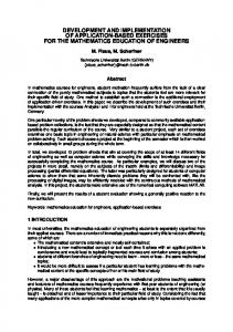
[Zaouche*, 5 (8): August, 2016] IC™ Value: 3.00 The created and 3D modeled aircraft F-16 is presented in the following figure.

ISSN: 2277-9655 Impact Factor: 4.116

Figure 1:

Model system “F-16.gmax”. The “FS2004 SDK Pack” is easily downloadable and contains many executable files such as “fs2004_sdk_gmax_setup.exe” and “makemdl_ sdk_setup.exe” that provide the possibility of compiling a “gmax” file to an FS-2004 exploitable “mdl” file. The gmax SDK (Software Development Kit) contains five separated SDKs, bundled together in one downloadable and installable file. When we install the “fs2004_sdk_gmax_setup.exe” in the gmax installation folder, we get the following tools and documentation: gmax_AttachTool, gmax_Animation, gmax_ CloudTool, gmax_Aircraft and gmax_Scenery. Once the “gmax gamepack SDK” is installed the created model can be exported to flight simulator by selecting "Flightsim aircraft object (*.MDL)" type when exporting. System’s dynamic model The aircraft aerodynamic model identification is treated in [7] and [14] by using the wind tunnel (see figure 2). The derivative aerodynamic coefficients obtained in [7] and [14] are used to validate our aircraft model F-16. Figure 2:

Photograph of 0.1 O-scale F-l6 mounted for large amplitude pitching tests in wind tunnel [7] and [14].

http: // www.ijesrt.com© International Journal of Engineering Sciences & Research Technology [34]

[Zaouche*, 5 (8): August, 2016] ISSN: 2277-9655 IC™ Value: 3.00 Impact Factor: 4.116 The “SDK FS2004” (Software Development Kit) describes with details the aircraft container system, explaining how the different files work together. It provides information on how to modify and share components among existing aircraft. It does not explain how to create a new aircraft. The “aircraft.cfg” is the configuration file for the aircraft. It is easily editable and the most important file for the user. The structure of this file is as follows:  It contains a text block of information which is directly related to aircraft behavior and contains data (external parameters) for the flight dynamics, in addition to those in the “*.air” file (internal parameters);  It contains a second block with information about all the liveries of that aircraft type. Figure 3:

Exported aircraft F-16 flying in FS-2004.

IDENTIFICATION PROCEDURE PART Structuring the Aerodynamic Data Base Aerodynamic Models The aerodynamic data are expressed in terms of three forces (drag X , lift Z , side force Y ) and three moments (pitching moment M , rolling moment L , yawing moment N ) that act on the aircraft. Next, the effect of dynamic pressure and aircraft size (expressed in terms of wing area , and mean aerodynamic chord or wing span ) is eliminated through working with dimensionless aerodynamic forces and moments coefficients [8], [13], [9], [5],[10]. (1) X Z Y CX 

,C Z  ,CY  1 1 1 V 2 S V 2 S V 2 S 2 2 2 L M N Cl  , Cm  , Cn  1 1 1 2 2 V Sb V Sc V 2 Sb 2 2 2

(2)

where; V : true air speed m ,  : air density Kg s

m

. 3

The aerodynamic coefficients C X C n , in (1) and (2) are functions of the time histories of the aircraft state, i.e. angleof-attack  ,

angle-of-sideslip  ,

the

aircraft

rotation

rates p , q , r

as

well

as

the

control

surface

deflections  e ,  a ,  r . The functional relationship between the aerodynamic coefficients and the state variables are expressed in terms of Taylor's series expansions about a reference state. A representative example is [5], [9], [10],[11], [13], [18]:

http: // www.ijesrt.com© International Journal of Engineering Sciences & Research Technology [35]

[Zaouche*, 5 (8): August, 2016] IC™ Value: 3.00

ISSN: 2277-9655 Impact Factor: 4.116

 qc C X  C X 0  C X    C X 2  2  C Xq  C X e  e  C X 0 Fp F p  V  CY  CY  CY   CYp pb  CYr rb  CY  a  CY  r  CYF  F p 0 a r p  2V 2V  qc C Z  C Z 0  C Z   C Zq  C Z e  e  C Z F  F p   V   C l  C l  C l   C lp pb  C lr rb  C l  a  C l  r  C lF  1 F p 0 a r p  2V 2V  qc C m  C m0  C m   C mq  C m e  e  C mF F p  V   C  C  C   C pb  C rb  C   C   C F n n0 n np nr n a a n r r nFp p  2V 2V 

(3)

where, CZ  

CZ C , CY   Y   ,

 1  ycg  y jet ,   z cg  z jet 

x jet , y jet and z jet are the positions of the specific force sensors.

Table 3. Aerodynamic coefficients Aerodynamic coefficient

Description

CX :

Axial force coefficient (body frame)

CX 0

:

C X

:

Drag at zero angle of attack and sideslip Drag due to the angle of attack. Angle of attack will increase the area facing the wind and therefore increase the drag Side force (body frame) Cross-wind force due to the sideslip. Sideslip will expose one side of the fuselage to the wind causing a net force in the Y direction Normal force coefficient (body frame)

CY : CY

:

CZ :

CZ 0

:

CZ

:

Cl , C m , C n

Lift at zero angle of attack. This will be non-zero for asymmetric airfoils Lift due to the increased angle of attack. The airfoil will generate greater lift as the angle of attack increases until the wing stalls Roll, pitch, yaw moment coefficients;

Clp

:

Damping from angular velocity. Mainly caused by the main wing when rolling

C l a

:

Roll moment due to aileron control surface deflection

Cl

:

C m

:

C mq

:

Restoring roll moment due to the sideslip. Mainly caused by the dihedral angle of the wing and the vertical stabilizer Restoring pitch moment due to the angle of attack. The tail horizontal surface will be the main contributor to this moment as it will hit the wind with an angle and thus generate the restoring moment Damping from angular velocity. Mainly caused by the vertical stabilizer when yawing

C m e

:

Pitch moment due to the elevator surface deflection

C n

:

Pitch damping coefficient

C nr

:

Restoring yaw moment due to the side slip. Vertical stabilizer at the tail will generate a restoring moment because of the exposed area while side slipping Yaw moment due to the rudder control surface deflection

C n r

http: // www.ijesrt.com© International Journal of Engineering Sciences & Research Technology [36]

[Zaouche*, 5 (8): August, 2016] ISSN: 2277-9655 IC™ Value: 3.00 Impact Factor: 4.116 There is a verification model that matches the aerodynamic coefficients to the measurements provided by the sensors of the aircraft. m  ax cos  cos   a y sin   az sin  cos    Fp cos  m cos  m  1  SV ² 2 qc C X 0  C X   C X  2  2  C X Q  CX  e e V m   ax sin   az cos    Fp sin  m qc  CZ0  CZ   CZQ  C Z  e e 1 V  SV ² 2 m  ax cos  sin   a y cos   az sin  sin    Fp cos  m sin  m  1  SV ² 2 pb rb CY0  CY   CYP  CYR  CY  a  CY  r  r a 2V 2V pI xx  q. p  I zz  I yy    p.q  r  I xz  1  SbV ² 2 p.b r.b Cl0  Cl   Clp  Clr  Cl a  a  Cl r  r 2V 2V qI yy  r. p  I xx  I zz    p ²  r ²  I xz  FP 1  ScV ² 2 q.c  Cm0  Cm   Cmq  Cm E  e V rI zz  q. p  I yy  I xx    r.q  p  I xz 1  SbV ² 2 p.b r.b  Cn0  Cn   Cnp  Cnr  Cn a  a  Cn r  r 2V 2V

(4)

a x , a y , a z are the linear acceleration components.

In this case the actual time series of the aerodynamic coefficients are not directly obtained from the simulator, but calculated based on typical aircraft instrumentation. The instruments are in this case, assumed to provide noise and bias free perfect measurements. This does not mean that systematic errors are not included and simulations will demonstrate how the corrections affect the results. Table 4 shows the used aircraft sensors.

Sensor Accelerometer Rate gyro Alpha vane Beta vane Pitot-static tube Aileron sensor Elevator sensor Rudder sensor

Table 4. Sensors used for obtained measurements Measured value Description Acceleration in body coordinates. a x , a y , az p, q, r

  Q

a e

r

Angular velocity in body co- ordinates. Angle of attack sensor. Measures the flank angle. Measures dynamic pressure. Aileron deflection angle. Elevator deflection angle. Rudder deflection angle.

http: // www.ijesrt.com© International Journal of Engineering Sciences & Research Technology [37]

[Zaouche*, 5 (8): August, 2016] IC™ Value: 3.00

ISSN: 2277-9655 Impact Factor: 4.116

IMPLEMENTATION OF A REAL-TIME INTERFACE BETWEEN MICROSOFT FLIGHT SIMULATOR AND “THE REAL TIME WINDOWS TARGET” MODULE OF SIMULINK/MATLAB We design our Software to interface the simulated aircraft in Flight Simulator environment (read and/or write many sensors, actuators data and parameters). Figure 4:

Block diagram of the software environment design. We communicate with FS2004 by using a dynamic link library called FSUIPC.dll (Flight Simulator Universal Inter Process Communication). This library created by Peter Dowson is downloadable from his website (www.schiratti:com/Dowson.html) [16], and can be installed by being copied in the directory (module) of FS2004. It allows external applications to read and write in and from Microsoft Flight Simulator MSFS by exploiting a mechanism for IPC (Inter-Process Communication) using a buffer of 64 Kb. The organization of this buffer is explained in the documentation given with FSUIPC, from which the Table II is taken. To read or write a variable, we need to know its address in the table, its format and the necessary conversions. For example, the indicated air speed is read as a signed long S32 at the address 0x02BC. Adress 6010 6018 6020 057C 0578 0578 30B0 30A8 30B8 3060 3068 3070 0842 02BC 2ED0 2ED8 0BB2 0BB6 0BBA 088C

Table 5. Flight parameters in the buffer FSUIPC Name Var.Type Size (octet) Latitude (λ) FLT64 8 Longitude (µ) FLT64 8 Altitude (h) FLT64 8 Bank angle () S32 4 Elevation angle (θ) S32 4 Head angle (ψ) U32 4 Rotation rate (p) FLT64 8 Rotation rate (q) FLT64 8 Rotation rate (r) FLT64 8 Acceleration (ax) FLT64 8 Acceleration (ay) FLT64 8 Acceleration (az) FLT64 8 Vertical speed (Vz) S16 2 Speed IAS (V ) S32 4 Incidence (α) FLT64 8 Incidence (β) FLT64 8 Elevator deflection (δe) S16 2 Aileron deflection (δa) S16 2 Rudder deflection (δr) S16 2 Thrust control (δx) S16 2

Usage Degree Degree Meter Degree Degree Degree rad/s rad/s rad/s ft/s2 ft/s2 ft/s2 meter/min Knot*128 Radian Radian -16383 to +16383 -16383 to +16383 -16383 to +16383 -16383 to +16383

http: // www.ijesrt.com© International Journal of Engineering Sciences & Research Technology [38]

[Zaouche*, 5 (8): August, 2016] IC™ Value: 3.00

ISSN: 2277-9655 Impact Factor: 4.116

TOTAL LEAST SQUARES ESTIMATION (TLSE) METHOD FOR AN AIRCRAFT AERODYNAMIC MODEL IDENTIFICATION Total Least Squares (TLS) is an extension of the usual Least Squares method: it allows dealing also with uncertainties on the sensitivity matrix. In this paper the TLS method is analyzed with a robust use of the SVD decomposition technique, which gives a clear understanding of the sense of the problems and provides a solution expressed in closed form in the cases where a solution exists. We discuss its relations with the LS problem and give the expression for the parameters governing the stability of the solutions. At the end we present the algorithm for computing , solution of the estimated aerodynamic coefficients problem [5],[10],[11] [19]. The aerodynamic model is expressed as follows: (5) Y  A.   



Both the vector of the variable-to-be-explained and certain columns of the matrix of explanatory variables stem from measurements which are subject to measurement errors. Under these circumstances, a clear distinction between true values and measured data must be made, (6) Am Y m   A0 Y 0  A0 Y 0  Where, index is used to indicate the measurements, index 0 is used to indicate the true values, and prefix m is used to indicate measurement errors. This is accomplished through rewriting the linear model of Equation (9) as, (7) A Y .1  0   Notice that the following linear relation is valid for the true data but will, in general, not be valid for the measured data,

A

0

A

m

  Y0 . 0   0   1   Y m . m   0  1

(8)



The Singular Value Decomposition (SVD) of the compound data matrix is defined by [5],[10],[11]:

A

m

Ym



1     2     .   . V T U   .    n1                  0  

(9)

The last and smallest singular value indicates the Frobenius norm distance of matrix to the nearest rank deficient matrix. With this knowledge, the estimates of the (most probable) minimum norm data correction matrix and the (most probable) corrected data matrix are,

http: // www.ijesrt.com© International Journal of Engineering Sciences & Research Technology [39]

[Zaouche*, 5 (8): August, 2016] IC™ Value: 3.00

ISSN: 2277-9655 Impact Factor: 4.116

 0    0     .   . V T Aˆ  yˆ  U    0    n 1                  0  





 1     2     .   . V T Aˆ Yˆ  U    n   0                 0  





(10)

(11)

An estimated of the (most probable) extended and transformed parameter vector must satisfy the equation, ˆ T (12) ˆ ˆ 

A Y  . 1  0 



Or,



ˆ     . ker Aˆ  1

yˆ



(13)





where  is a scalar multiplier used to make the last element of v n1 equal to -1. The kernel of matrix Aˆ Yˆ equals the last right singular vector v n 1 . In our case, the Measurement vector Y is defined as follows: Y  C X

CY

CZ

Cl

Cn 

T

Cm

 Y1 Y2 Y3 Y4 Y5 Yn 

61

(14)

T

Y1  Y2  Y3  Y4  Y5  Y6 

ma x cos cos   a y sin   a z sin  cos    Fp cos m cos  m 0.5 SV ² m a x sin   a z cos   Fp sin  m 0.5 SV ² m a x cos sin   a y cos   a z sin  sin    Fp cos m sin  m

(15)

0.5 SV ² p I xx  q. p I zz  I yy    p.q  r I xz 0.5 SbV ² qI yy  r. pI xx  I zz    p ²  r ² I xz   .Fp 0.5 Sc V ² rI zz  q. p I yy  I xx   r.q  p I xz 0.5 SbV ²

We note that there is no sensors which provide the angular accelerations p , q and r . We used a differentiator for their computation [5],[10],[11]:

http: // www.ijesrt.com© International Journal of Engineering Sciences & Research Technology [40]

[Zaouche*, 5 (8): August, 2016] IC™ Value: 3.00

ISSN: 2277-9655 Impact Factor: 4.116

A is the 6 37 dimensional matrix of explanatory variables, and  is the 371 dimensional vector of system 

parameters. Where, A  A1 A2 A3 6 x 37  2  0 0 0 0 0   0  0 0 0 0 0   0 0  0 0 0 0 A1   0 0 0  0 0 0   0 0 0 0  0 0    0 0 0 0 0  0 1 0  0 A3   0 0  0

(16) qc V

0

0

pb 2V

0

0

0

0

0

0

0

0

0

0

0

0

0

0 0

0

0

pb 2V

rb 2V

0

0

0

0

0

0

0

qc V

0

0

pb 2V

0

0

0

0

0

0

0

0

F p

0

0

0

0 1 0 0 0

0

0

F p

0

0

0 0 1 0 0

0

0

0

 1 Fp

0

0 0 0 1 0

0

0

0

0

F p

0 0 0 0 1

0

0

0

0

0

2

3

4 

0

qc V

0

  1

0

rb 2V

1 0 0 0 0

T

0

0

0

0 0 0 0 0 Fp

0

0

0

  e 0  0    0 0  A2    0 0   0  0   0   0  rb  2V  6 x16

0

0

0

0

0

0

0

a r

0

0

0

0

0

0

0

e

0

0

0

0

0

0

0

0

0

0

0

0

0

0

e

0

0

0

0

0

0

0

a

a r

0 0  0  0 0   r  6.9

0  0  0   0  0   F p  6.12

(17)

371

1  CX  CY  CZ Cl  Cm Cn CX  2 CXq CYp CYr CZq  2  Clp Clr Cmq Cnp Cnr CX e CYa CYr CZe Cla Clr 



 2  C m e C n a C n r C X 0 CY0 C Z0 Cl0 C m0 C n0 C XFp CYFp C ZF



RESULTS SIMULATION We run the Flight Simulator FS2004 and the interface with the module Real Time Windows Target of Simulink/Matlab. The aircrafts’ taking off were done using the keyboard. Several flight tests were conducted by changing the simulation parameters (season, time of day, weather). We present some recorded signals taken from the Inertial Measurement Unit (IMU). Figure 5: Accelerations

ax(m/s2)

10 0 -10 -20

0

100

200

300

400

500

600

700

800

0

100

200

300

400

500

600

700

800

0

100

200

300

400 500 N° Samples

600

700

800

ay(m/s2)

20

0

-20

az(m/s2)

20 0 -20 -40

Accelerations m/s2.

http: // www.ijesrt.com© International Journal of Engineering Sciences & Research Technology [41]

[Zaouche*, 5 (8): August, 2016] IC™ Value: 3.00

ISSN: 2277-9655 Impact Factor: 4.116 Figure 6: Rotation rates 1

p(rd/s)

0.5 0 -0.5

0

100

200

300

400

500

600

700

800

0

100

200

300

400

500

600

700

800

0

100

200

300

400 500 N° Samples

600

700

800

q(rd/s)

1

0

-1

r(rd/s)

0.5

0

-0.5

Rotation rates rd/s. The estimation of the aerodynamic parameters is performed with TLSE method. Fig. 7 shows the measured and estimated values of the longitudinal force coefficient C X , the vertical force C Z , and the pitching moment coefficient C m . Figure 7: Aerodynamic coefficients xest

0.5

and C

Cxest Cxmes

C

xmes

0

and C

zest

-0.5

100

200

300

400

500

600

700

1 Czest

0

zmes

C mest

and C

mmes

C

0

Czmes

-1 -2

0

100

200

300

400

500

600

700

0.02 Cmest

0.01

Cmmes

0 -0.01

0

100

200

300 400 N° Samples

500

600

700

Measured and estimated aerodynamic coefficients

http: // www.ijesrt.com© International Journal of Engineering Sciences & Research Technology [42]

[Zaouche*, 5 (8): August, 2016] ISSN: 2277-9655 IC™ Value: 3.00 Impact Factor: 4.116 The Fig. 8 shows the measured and estimated values of the rolling moment coefficient C l and the yawing moment coefficient C n : Figure 8: Aerodynamic coefficients

lest

0.01 Clest

and C

0

Clmes

lmes

-0.01

C

-0.02 -0.03

0

100

200

300

400

500

600

700

-3

x 10

5

Cnest

and C

nest

0

Clmes

-5

C

nmes

-10 -15 -20

0

100

200

300 400 N° Samples

500

600

700

Measured and estimated aerodynamic coefficients. Finally, the goodness of fit the model can be expressed in terms of a correlation coefficient between Y and Y est . This coefficient is usually referred to as the multiple correlation coefficient whose square is:

Y  Y  Y  Y  ;  Y  Y  Y  Y  T

R

2

est

est

T

1 N

Y



N

Y

i 1 est

i 

(18)

In general, the estimated values of C Xest , C Zest and Cmest fit well with the measured values. The total correlation coefficient R2, see equation (18), of the force and moment coefficients are 0.1337, 0.9777 and 0.927 respectively. The value of the multiple correlation coefficient R can be as high as one when the model fit is perfect, or zero when no correlation exists between the estimated and the measured dependent variable Y. The obtained results show that it is possible to identify at the same time the whole set of the aircraft aerodynamic coefficients derivatives by using the TLSE method (see Fig. 9). Figure 9: -3

Aerodynamic coefficients derivatives

C

xalpha

x 10 2 0 -2 -4

C

xsigmae

0

100

200

300

400

500

600

700

0.05 0 -0.05 0

100

200

300

400

500

0

100

200

300 400 N° Samples

500

600

700

C

ysigmae

0.05 0 -0.05 -0.1 600

700

Estimated aerodynamic coefficient derivatives

http: // www.ijesrt.com© International Journal of Engineering Sciences & Research Technology [43]

[Zaouche*, 5 (8): August, 2016] IC™ Value: 3.00

ISSN: 2277-9655 Impact Factor: 4.116

CONCLUSION In this paper, procedures of the creation, the 3D modeling and the integration of an aircraft model in simulated environment have been explained. After that, the aircraft aerodynamic aspect for Microsoft Flight Simulator has been presented. Our approach uses the environment simulator (FS2004) to reduce the design process complexity. Particularly, we are interested in the flight tuning section in the “aircraft.cfg” file, which treats the aerodynamic part. In this section, we realize that the aerodynamic coefficients derivatives are unknown and not afford by MSFS 2004. The only provided numerical values (default 1 in most cases) are multipliers to the aerodynamic coefficients derivatives. We have presented the Total Least Square Estimators Method (TLSE) applied to the aerodynamic identification problem. This method is based on the use of the SDV decomposition. It has the interesting propriety of giving the best approximation of the augmented measurement matrix, by another matrix with the same dimension, but with a lesser range, in the sense of the least squares. The aerodynamic parameter in the model has been estimated based on flight data using the TLSE method. The parameters identification results show a good match between the estimated and measured values.

REFERENCES [1] Harkegard O. Flight Control Design Using Backstepping. LINKOPINGS UNIVERSITET, LINKOPING, SWEDEN, 2001. [2] Feldstein C.B., Muzio J.C. Development of a fault tolerant flight control system. 23RD DIGITAL AVIONICS SYSTEMS CONFERENCE IEEE, PP. 6.E.3 - 61-12 VOL.2, 2004. [3] Louali R., Belloula A., Djouadi M.S., Bouaziz S. Real-time characterization of Microsoft Flight Simulator 2004 for integration into Hardware In the Loop architecture. 19TH MEDITERRANEAN CONFERENCE ON CONTROL AND AUTOMATION (MED), PP. 1241-1246, 2011. [4] Microsoft Flight Simulator 2004 and FSX. https: //www.microsoft.com /enus/download/ details.aspx ?id=9 727, 2009. [5] Zaouche M., Beloula A., louali R., Bouaziz S., Hamerlain M. Adaptive differentiators via second order sliding mode for a fixed wing aircraft. COMPUTER MODELING IN ENGINEERING AND SCIENCES.VOL.104, NO.3, 2015. [6] Microsoft developer network. https://msdn.microsoft.com/enus/library/cc526949.aspx. MICROSOFT CORPORATION, 2008. [7] Klein V., Murphy P.C., Curry T.J., and Brandon J.M. Analysis of Wind Tunnel Longitudinal Static and Oscillatory Data of the F-16XL Aircraft. NASA/TM-97-206276, 1997. [8] Golub Gene H., Van Loan Charles FMatrix computations. 4TH EDITION, THE JOHNS HOPKINS UNIVERSITY PRESS BALTIMORE, . 2013. [9] Roskam Jan. Airplane flight dynamics and automatic flight controls, part I. DARCORPORATION, 2001. [10] Zaouche M. Identification et commande robuste d’un engin aérodynamique volant à 03 axes», THESE DOCTORAT, ECOLE MILITAIRE POLYTECHNIQUE, ALGIERS, 2015. [11] Zaouche M., Amini M., Foughali K., Aitkaid S., Bouchiha N.S. Application of the total least squares estimation method for an aircraft aerodynamic model identification. INTERNATIONAL JOURNAL OF MECHANICAL, AEROSPACE, INDUSTRIAL, MECHATRONICS AND MANUFACTURING ENGINEERING. VOL 10, N°06, PP.1067-1076, 2016. [12] Adiprawita W., A. S. Ahmad, J. Semibiring, Hardware In The Loop Simulator in UAV Rapid Development Life Cycle. ICIUS, BALI, INDONESIA, 2007. [13] Anderson John D. Aircraft performance and design», MCGARW-HILL, 1999. [14] Brandon Jay M. and Foster. John V. Recent dynamic measurements and considerations for aerodynamic modeling of fighter airplane configurations. AMERICAN INSTITUTE OF AERONAUTICS AND ASTRONAUTICS, AIAA - 98-4447, 1998. [15] Boiffier Jean-Luc. The dynamics of flight: The equations. JOHN WILEY AND SONS, 1998. [16] Dowson P. FSUIPC: Application interfacing module for Microsoft Flight Simulator. Available online at: www.schiratti.com/dowson.html, 2012. [17] Gimenes R., Castro Silva D., Paulo Reis L and Oliveira E. Flight simulation environments applied to agentbased autonomous UAVs. INTERNATIONAL CONFERENCE ON ENTERPRISE INFORMATION SYSTEMS, 2008. http: // www.ijesrt.com© International Journal of Engineering Sciences & Research Technology [44]

[Zaouche*, 5 (8): August, 2016] ISSN: 2277-9655 IC™ Value: 3.00 Impact Factor: 4.116 [18] Laban M. On-Line Aircraft Aerodynamic Model Identification. PHD DISSERTATION, TECHNISCHE UNIVERSITEIT DELF, 1994. [19] Markovsky Ivan, Huffel Sabine Van. Overview of total least-squares methods. SIGNAL PROCESSING, SCIENCE DIRECT, 2007.

http: // www.ijesrt.com© International Journal of Engineering Sciences & Research Technology [45]