Development of a Dynamic Simulator for Braking Performance Test of Aircraft with Anti-skid Brake System Jeong-Woo Jeon, Ki-Chang Lee, Don-Ha Hwang and Yong-Joo Kim Mechatronics Research Groups, Korea Electrotechnology Research Institute, P.O. Box 20, Changwon, Kyungnam, Korea email:
[email protected] Absnacr- In this paper, the dynamic simulator with 5-D.O.F. aircraft dynamic model and ABS control hiw unit with ABS control algorithm are developed and are tested to depend on some conditions of gripping coefficient. ABS control hiw unit on wet or snowy runway as well as dry runway v e n well protects wheel sliid. 1. INTRODUCTION
ABS (Anti-skid Brake System) has been applied to railways since the beginning of the 20th century. An application of ABS was extended to automobiles and aircrafts. ABS for aircrafts is for braking security, braking distance shortening as well as a protection against wheel skid. A general anti-skid control method employs a digital control unit to detect a velocity of main landing wheel. The digital control unit decides a skid condition of the wheel and it protects the skid condition by controlling pressures ?I brake cylinders. In this paper, the dynamic simulator that was developed for brake performance test of aircraft with anti-skid system is introduced. The dynamic model is composed of a big contour and a little contour by simulation siw. The big contour represents the interactions of forces in airframe, nose and main landing gear, and engines on the center of gravity. The little contour represents interactions of wheel. braking units. hydraulic units and a control unit. Dynamic simulator simulates the dynamic model. Tbe configuration of dynamic simulator is shown in Fig. 1. The dynamic simulator is real-time interface system that is composed of dynamic simulation parts, master control parts, digital and analog idout interface parts, and user interface parts. The dynamic simulation part simulates 5-D.O.F. (Degree offreedom) aircraft dynamic model. The digital and analog idout interface part exchanges digital and analog data between dynamic simulator and digital control hiw unit. The user interface part transfers real-time commands from user to
dynamic simulator and graphical test results from dynamic simulator to user. The digital control unit is consmcted to accommodate the ABS control algorithm. The algorithm is verified by real-time closed loop test with dynamic simulator and the test results are presented. The purpose of this test method is to develop a digital control unit with ABS control algorithm using the aircraft dynamic model. The digital control unit is tested under various road conditions.
11. D Y ~ A M I C OF S AIRCRAFT LAXDING
In this paper, a dynamic model of 5-D.O.F. for aircraft landing is developed. The dynamic model is composed of a big contour and a little contour. A . The Big Conroiirs ofAixraj7 Dynamics
The big contour that is shown in F i g 2 represents the interactions of forces in airframe, nose and main landing gear and engines on the center of gravity [ 13.
Fig. 2. The big contour of aircraft dynamics 5-D.O.F. AUCraft
%sital and h a l o . Data
DpallliCS
IniOut inteface
MaWi
User
Control
1ntcrface
Dynamic Simulator
Fig. 1. The configuration of Dynamic Simulator
0-7803-7369-3/02/$17.000 2002 IEEE
At the stage of braking in the process of landing, the aircraft is affected by the forces as follows: aircraft gravitational forces, total aerodynamic forces, total engine thrust forces and total landing gear response forces when moving by the runway surface. The total aerodynamic force is applied at the aircraft center of gravity. The airframe is considered as a rigid beam with mass localized in the center of gravity, it is loaded by the aircraft system of aerodynamic forces and moments (X", Z", MA),total aircraft engine thrust forces and moments (XE,ZE,ME),nose landing gear response forces and moments (X"2, Zns, M"') and main
518
b, - Characteristic length, m landing gear response forces and moments (X"', Zms,Mm8)). S,,, - Wing area, m' The airframe model that is shown in Fig.3 represents a vertical motion, a horizontal motion and a rotating motion on center of gravity as well as rotating motions of nose and main C. Aircrafi 61ginr Thrmt (y,Z". hf) landing gear. The aircraft landing along the runway is performed with maximum use of all brake means. Besides the brakes of the landing gear wheels, these means incorporate the jet and turbojet engines' reversing devices. The horizontal and vertical projections of the aircraft engine thrust vector of the earth coordinate axes and its pitch moment are described by equations: Fig. 3. The airframe model
X E= Fc0sa.n Z' = F s i n a . n
(7)
M E = FLn
(9)
The airframe dynamic model is described by the system of 6-order differential equations as follows [?I:
(8)
F -Aircraft engine transient force, N a -Angle of aircraft engine thrust vector action n - Number of aircraft engines L - The ann of the aircraft engine thrust vector, m
D. Forces and Moments of The ruse Landing Gears (P, Z ' F , ,&,fOD)
x. z - Horizontal and vertical coordinates of the airframe center of gravity in the earth coordinate system, m 0 -Pitch angle. rad g - Free fall acceleration. ids' mpl-Airframe mass; kg JPI - Airframe main central moment of inertia relative to the lateral axis, Nnis'
Nose landing gear is shown in Fig.4. It takes account of statically non-linear characteristic of the nose landing gear shock-absorber con~pression and the shock-absorber damping features. The projections of responses are calculated according to expressions as follows:
s,:
-
X" = X: cosy -z:sin y
(4)
Z" = X : s i n y + Z : c o s y
(5)
(10)
ZjiS= F,,,, COS 6
(11)
M "OD
=X
"E
z + Z "E Xr9
(12)
B - Airframe pitch angle, rad Fa,- Shock-absorber force, N p - Coefficient of rolling friction, ni ,C,,s -Abscissa of the MLG attaching point. m / s
B. Aer-o&nan?ic Fovces and Monienfs (x'.2 ''. &)
After lowering the nose landing gear the spoiler tum on takes place. Spoilers are one of the means of aircraft brake during the mn, which increase the aircraft resistance and decrease the lift value. The horizontal (XA)and vertical (Z') projections of aerodynamic forces on the earth coordinate axes and the aerodynamic pitch moment (MA) relative to the airframe center of gravity are described by non-linear equations:
X"-$ = F,,,(sine+pcos6)
E. Forces arid Munients of The Main Landing Gears (x"?
z"%,M"S)
Main landing gear also is shown in Fig.4. It takes account of statically non-linear characteristic of the main landing gear shock-absorber compression and the shock-absorber damping features. The projections of responses are calculated according to expressions as follows:
z"'* = F,,, cos e M n's = x zw
Aerodynamic force of head resistance, N
mg
z; - Aerodynamic lift, N y - Aircraft path slope, rad C, - Aerodynamic coefficient of the pitch moment
04)
+
"'E
xmp- Abscissa of the MLG attaching point, d s
519
(15)
a,, -Braking wheel angular velocity U,!
-Angular velocity of non-braking wheel
Fig. 4. The landing gear F. The Little Contoiris (Wheel Brake Assav Confruller)
I
The little contour that is shown in Fig.5 represents interactions of wheel, braking units, remote pressure control system (RPCS) and ABS control unit.
p a
Fig. 6 . Reflection force on contact between a wheel and a runway
Fig. 5 . The little contour (Wheel Brake Assay. Controller) The control signal is fed on the RPCS input and then the brake pressure is fed on the brake and then the feed hack signal that measured brake pressure values is fed on the controller. The braking moment from the brake is fed on the wheel and then the angular velocity from the wheel is fed on the controller. Braking wheel forces are transferred into the big contour. The controller detects skid of wheel and then generates control signal for anti-skid control. G. Forces on The Wheel A reflection force on contacts between a wheel and a runway is shown in Fig.6. Here, The Fbis brake force and the F, is friction force. This forces affects landing gear dynamic model in big contour. The friction force of the wheel are described by equations [3]:
F,
= p,Z
In running of wheel on surface, if brake force is increased, the velocity of wheel is decreased and then slip is increased and then gripping coefficient is increased and then friction force is increased. If brake force is more increased, the velocity of wheel is more decreased and then slip is more increased. If slip is higher then S I , gripping coefficient is decreased and then friction force is decreased. Here, if friction force is lower than braking force, the velocity of wheel is quickly decreased and then slip is quickly increased and then friction force is quickly decreased. In consequence wheel is locked and skidded. The gripping coefficient is affected by runway. If runway is dry, the maximum value of grippingcoefficient(pm,,)isabout0.7-0.8. lfrunway is wet or snowy, the maximum value is about 0.2 0.3. In this paper, the curves of gripping coefficient (ps) are presented like Fig.7-IO. These graphs are not real but similar. Generally. if slip ratio is between 0.05 and 0.2, the gripping coefficient (pJ is maximum value. ~
H. The Remote Pressure Control Sisfeni Model The RPCS is composed by electro-hydraulic control valve, pipeline and hydraulic cylinder like Fig. 1 1. Depending on the problem being solved, the mathematical models used in the design of the hydraulic drive static and dynamic characteristics may have various complexities. More simple models of the hydraulic drive are used for the study of the entire aircraft control system. The flow rate in the hydraulic cylinders of the brake is defined by equation:
Q,,
(16)
= sbr-+br
08)
Sbr- The area of the hydraulic cylinder piston, m' .eb, Displacement of the hydraulic cylinder piston, d s
ps- Coefficient of the runway surface grip of the wheel (gripping coefficient) Zmz- The wheel radial road, N The gripping coefficient is affected by slip(s) like Fig.7. The slip is described by equations:
~
The piston dynamic model in cylinder may he described
520
by the second-order equation:
ordinary non-linear
m b r i+ hb,.ibr= F, ( p b r mh, -The I,#,
differential
- F2(xb,) - R,,
(19)
mass of the brake movable parts
- The factor, taking account of the viscous friction
~ , ( p , ) - Non-linear
brake pressure dependence of the in brake force F:(x~,) Brake disk placement non-linear dependence of the frictional force Norman component in the brake disks R ~ -Dry , ~ friction force ~
1
0 5
Fig. 8. Gripping coefficient on pmnx= 0.6
Fig. 1 1. The remote pressure control system The flow rate at the pipeline inlet in equation (20) for the first section is expedient to the described as a function of displacement of the electro-hydraulic control valve: I
1
0 s
Fig. 9. Gripping coefficient on pmxy = 0.4 - Displacement of the electro-hydraulic control valve, mm f ( x ; ) - Electro-hydraulic control valve flow rate characteristic Pnr - Hydraulic system pipeline pressure, psi p , -Evaporation pressure, psi
,y,
I. The Braking Monient Model
0 1
0 S
Fig. I O . Gripping coefficient on pmar = 0.2
The brake simulation model represents hysterics of brake static characteristic, dynamic loss at pressure feed and release. Fig.12 shows hysteretic loop of brake characteristics.
521
A
L
Fig. 13. Situation logics of4El and SEI
I
Brake Pressure [PSII
Fig. 12. Hysteretic loop of brake characteristics
111. ABS COZTROL UN11
I
I
,,..
Fig. 14. Example of applying the situations
A . ABS ConfrolAlgol-ithm
The control algorithm determines presentation of control unit's output signals depending on incoming signals and commands during operation o f the unit in brake mode. Several situations (or Events) are defined to depend on conditions of incoming signals and commands in brake mode on runway. The ABS control hiw unit determines a situation and then generates a control signals. The situations for ABS control algorithm are shown in Table 1. The ABS control algorithm is composed of 10 situations. Situations of brake prohibition depending on aircraft conditions are IE, ?E and 3E. Situations of braking operation depending on deceleration and slip ratio are 4E and 5E. These logics are occurred as Fig. 13. If the hysteric's band is not, some errors are occurred at transition point and then reliabilities are bad. Situation of pressure drop to initial pressure is 6E. Situation of slowing down pressure is 7E. Situation of finishing pressure drop is 8E. Situation of slowing up pressure is 9E. Situation of increasing pressure is IOE. An example of applying the situations is shown in Fig. 14.
I
1 E. ABS Coiifrol H/W Unif
The ABS control algorithm is applied to ABS control hiw unit for anti-skid control. The main processor of ABS control hiw unit is TMS320C240-20MHz. The control unit has analog 110 to interface speed sensor, pressure sensor and etc as well as digital IiO to interface ZBVDC-relays. The specifications of ABS control hiw unit are shown in Table 2. Table 2. Specification of ABS control hiw unit
Control Penod