Proceedings of COBEM 2003 COBEM2003 - 0451 Copyright © 2003 by ABCM
17th International Congress of Mechanical Engineering November 10-14, 2003, São Paulo, SP
DEVELOPMENT OF A DYNAMIC POSITIONING SYSTEM SIMULATOR FOR OFFSHORE OPERATIONS Eduardo Aoun Tannuri Tiago Turibio Bravin Naval Architecture and Ocean Engineering Department, Escola Politécnica, University of São Paulo
[email protected]
Celso Pupo Pesce Mechanical Engineering Department, Escola Politécnica, University of São Paulo This paper describes a computational simulator for Dynamic Positioning Systems (DPS) under development in a R&D project carried out at USP and Petrobras. The simulator comprises models for main DPS sub-systems, namely control logic, filtering, thrust allocation and propulsion. It enables the simulation of several DP operations, as drilling station keeping, pipe laying path following and those related to assisted offloading. In order to address the performance of commercial DPS, two conventional control algorithms were implemented, namely a 3-axis uncoupled PID and a Linear Quadratic (LQ) controller. Since DPS should not compensate first-order wave force induced motions, measurement of position and heading must be filtered. This task is usually done by a notch filter or a Kalman estimator. In the present simulator both were considered. The simulator also considers fixed and azimuth-free propellers modeling, taking into account their own dynamics and time response characteristics. In conventional DPS, thrust control can be carried out either by controllable pitch mechanisms or through rotation control, both models being implemented in the simulator. Finally, the thrust allocation algorithm is included, minimizing fuel consumption. Some illustrative examples are presented in the paper, highlighting some of the main characteristics of the simulator. Keywords. Dynamic Positioning Systems, Control, Filtering, Offshore operation.
1. Introduction In recent cooperative R&D projects, University of São Paulo (USP) and the Brazilian oil-state company (Petrobras) developed a complete computational simulator for offshore system dynamics evaluation. The simulator, named Dynasim, can treat multiple body systems, such as offloading shuttle-FPSO-monobuoy configurations, taking into account risers and mooring line effects (Fig.1). It comprises several models for environmental forces (current, wind and waves), and is able to analyze 6 degrees of freedom per body. Several experimental and numerical validations have been conducted and, nowadays, Dynasim is considered an important tool for design and analysis in Brazilian oil industry (Nishimoto et all, 2001).
Figure 1. Dynasim – (center) offloading operation; (bottom) crane and pipe-launching barge; (up) mooring system and risers representation; (left and right) position time series and mooring line characteristic curves. Originally, Dynasim was designed to simulate moored vessels, subjected to environmental agents, without any propeller force. Further demands from Petrobras required USP to expand Dynasim capacities, implementing the possibility of simulating Dynamic Positioning Systems (DPS). Such kind of systems has been used extensively by the offshore industry, applied to several operations, as drilling, pipe laying, surveying and supplying. Conventional DPS keeps the vessel in close proximity to a required position in the horizontal plane, through the controlled application of forces generated by installed thrusters. A DPS comprises four sub-systems that must be taken into account during the development of a simulator (Bray, 1998). The first one is the power subsystem, responsible for the generation of energy delivered to thrusters, sensors and computers. Generation failures and blackouts are common problems of a DPS, and their consequences must be
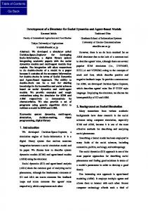
previously analyzed. Propellers and their local drivers and controllers, being responsible for the generation of the positioning thrusts compose the actuation subsystem. Two classes of propellers are broadly used in DPS, depending on the mechanism to obtain thrust variation. The controllable pitch propellers (cpp), which vary the thrust changing blade pitch, and fixed pith propellers (fpp), which vary the thrust by changing the rotation. The sensing subsystem is composed by all measurement devices, which are used to obtain reliable information about the vessel real position and heading. Wind and current sensors are also employed, in order to improve DPS performance. Finally, the control subsystem is composed by computers and algorithms, and is responsible to analyze information and to calculate the required forces in each propeller. Three main classes of algorithms are used in a DPS. A low-pass filter, called wave-filter, is employed to separate high-frequency components (excited by waves) from measurements signals. Such decomposition must be performed because the DPS must only control low-frequency motion, since high-frequency motion would require enormous power to be attenuated and could cause extra tear and wear in propellers. Furthermore, an optimization algorithm, called thrust allocation, must be used to distribute control forces among thrusters. It guarantees minimum power consumption to generate the required total forces and moment, positioning the vessel. At last, a control algorithm uses the filtered motion measurements to calculate such required forces and moment. Normally, a wind feedforward control is also included, enabling to estimate wind load action on the vessel (based on wind sensor measurements) and to compensate it by means of propellers. In order to address the performance of commercial DPS, two conventional control algorithms were implemented in Dynasim, namely a 3-axis uncoupled PID and a Linear Quadratic (LQ) controller. The feedforward wind compensator was also developed, since it is broadly employed in commercial systems. Two classes of wave filters were implemented: a conventional cascaded notch filter and a Kalman estimator. Finally, a thrust allocation algorithm, based on a pseudo-inverse matrix technique, was implemented, with extra features that are normally employed in real DPS. Three DP operation modes were considered in the simulator. The first mode is the conventional station-keeping mode, in which the desired position and heading (set point) are fixed. It is extensively used in drilling operations. Furthermore, a path-following mode was also considered, with a time-varying set point, commonly used in pipe-laying operations. Finally, offloading operations requires special control strategies, which were also implemented in Dynasim. The simulator also includes models for cpp and fpp propellers, taking into account their characteristics curves, being able to estimate real power consumption and delivered thrust. It also evaluates time delay between command and propeller response, caused by axis inertia (in case of fpp propellers). Different sensors and power generation models are not considered in the present simulator. This paper is organized as follows. Section 2 presents a brief description of wave-filters implemented in Dynasim. Section 3 details the thrust allocation algorithm and their extra features, which are illustrated by means of examples. Section 4 details the control algorithms and DP operation modes included in the simulator. Section 5 contains a description of propeller models. Section 6 presents three case studies, trying to illustrate some main features of the simulator. Section 7 draws some conclusions. 2. Filtering Wave filtering is an important algorithm in DP systems. Vessel motion is composed by high frequency components induced by first order wave forces and by low frequency components, causing large amplitude motions. Control system is responsible for controlling only the slow components, since the control of high frequency motions will damage propulsion system and would require enormous power to be attenuated. Therefore, motion measurements must be filtered, and only low frequency components must be fed back to the control system. Real time filtering involves a trade off between first order motion attenuation and the delay induced in the signal. This trade off fully affects the DPS performance. A perfect attenuation with a huge delay time or a minimum delay due to a weak attenuation compromises control performance. Whence, this trade off is mandatory in the simulator filtering development and implementation. Two different wave filters algorithms were implemented in the simulator. The first one is a modified classical DP filter design, presented by Grimble and Johnson (1989). Called Cascated Notch Filter, it associates three Notch filters, guaranteeing a broad frequency range attenuation that covers common wave induced motion frequency range. Its transfer function and Bode diagram is shown below: 3
H onda ( s) =
∏ i =1
s 2 + 2ζω i s + ω i2 (s + ω i ) 2
(1)
where ω1,ω2 and ω3 are the center frequencies of each notch filter and ζ is the relative damping factor. Typical values for the parameters are ω1=0.4rad/s; ω2=0.63rad/s; ω3=1.0rad/s and ζ=0.1.
M a gn itud e (d B )
Magnitude (dB)
0 -1 0 -2 0 -3 0 -4 0 20 0
Phase (deg)
Fa se (Gr a us)
10 0 0 -1 00 -2 00 10 -1
10 0
10 1
Frequency (rad/s) Frequê nc ia (rad/s)
Figure 2. Bode diagram of Cascaded Notch Filter This filter presents a good wave frequency attenuation with a delay of 8s. Simulations presented later show that such filter is appropriate for medium and large size vessels. The second filter implemented in Dynasim was a Kalman filter, based on simplified models for low frequency and high frequency motions of the vessel. The models adopted in the present work are based on Fossen (1994), with some simplifications. Being X and Y the position of the central point of vessel main section and ψ its heading angle, low frequency motion can be described by: 0 x& L = 3x3 0 3x3
I 3x3 0 x L + 3x3 −1 (FT + FE ) 0 3x3 M
, with x L = (X L YL ψ L X& L Y&L ψ& L )T
(2)
where FT are thrusters forces and moment vectors, FE are low frequency environmental forces and moment vectors and M is the mass-inertia matrix of the vessel (including hydrodynamic added masses). The subscript L is related to low frequency motion. In this model, the heading angle is considered to be smaller than 20o, approximately, during the motion. Viscous damping is neglected. The forces FE are slow varying unknown variables, and can be modeled by: (3)
F& E = ω L
where ω L is a 3x1 vector containing zero-mean Gaussian white noises processes with covariance matrix QL ( ω L ~ N (0, Q L ) ). Finally, high frequency motions can be modeled by: 0 3x3 x& H = 2 − ω 0 I 3x3
I 3x3 0 x L + 3x3 ω H − 2ζω 0 I 3x3 I 3x3
, with x H =
(∫ X
H
dt
∫Y
H
dt
∫ψ
H
dt
XH
YH
ψH
)
T
(4)
where ω H is a 3x1 vector containing zero-mean Gaussian white noises processes ( ω H ~ N (0, Q H ) ) and H represents high frequency. The parameter ζ is the relative damping ration of the motions, and was set as 0.1. The frequency ω0 is chosen as 0.5rad/s. The measured signals z are given by: X L + X H + vX z = Y L + Y H + vY ψ L + ψ H + vψ
(5)
where v is a 3x1 vector containing zero-mean, Gaussian white noise processes ( v ~ N (0, R ) ). Equations (2), (3), (4) and (5) were written as discrete-time state space models and applied to a standard Kalman Filter. The matrixes QL, QH and R are considered diagonal in the present work, and the correct tuning of their elements is briefly described later. It should be emphasized that the Kalman Filter estimates components xH and xL and also low frequency environmental forces FE. Kalman filter presents a complex formulation, requiring more sophisticated control algorithms and more advanced computer software. Besides, the tuning of matrix gains requires time-consuming trial and errors procedure. Here, the trade off between attenuation and delay time is also respected. With the matrix gains presented below, this filter works well, causing a time delay smaller than 8 seconds.
(
R = diag 1m 2 1m 2
(
(π / 180) 2 rad 2
)
4
QL = diag 0.1×10 (kN / s)2 1×10⁴ (kN / s)2 9 ×10⁶ (kN.m / s)2
(
Q H = diag 80(m / s) 2
80(m / s) 2
4 × 10 −2 (rad / s) 2
)
)
Nevertheless, as an extra result, Kalman Filter also estimates low-frequency environmental forces, what can be fed into feed-forward or adaptive control algorithms. Detailed description of both wave-filters and a comparison between them is presented in Tannuri et al. (2003). 3. Thrust Allocation The thrust allocation logic is responsible for delivering moment and forces calculated by control module algorithms. Such algorithms are oriented towards fuel consumption minimization. The implemented technique, described by Lewis (1986), is based on a pseudo-matrix inversion, explained below. T = ( A T A) −1 A T FT
(6)
where, FT=(F1T, F2T, F6T)T represents the control forces and moment assignments, and
A=
1 0 − x2,1P
.
1
0
.
0
c1+ nazim
.
0
1
.
1
s1+ nazim
. − x2,nazim P
x1,1P
(7) . s n prop . − cn prop .x2,n prop P + s n prop .x1,n prop P
.
− c1+ nazim .x2,(1+ nazim ) P + s1+ nazim .x1,(1+ nazim ) P
. x1,nazim P
cn prop
being ci = cos(α iP ) e si = sen(α iP ) , and αiP the azimuth angle when using azimuth propellers, xi the propeller position according to an orthogonal reference frame fixed to the vessel. The vector T brings surge and sway force components required in each available propeller, fixed or azimuth. The required azimuth and thrust are directly obtained from such components. A reallocation facility was also included in the simulator. It consists in reallocating the forces and moment exceeding the nominal power capability of one propeller, among others with available power. The thrust allocation algorithm calculates the difference between the total forces and moment required by the controller and the total force and moment delivered by propeller system. After that, it reallocates the difference among the propellers that are not saturated. It redoes the operation until all propellers are saturated or until no non-saturated propeller is available to be delivered with the required exceeding forces and moment. Figure 3 illustrates this feature. In (a) and (b) Figure 3 presents, respectively, the sway force and yaw moment required by a fictitious control system. These force and moment must be produced by the azimuth propeller system of a dynamically positioned barge, presented in (c) (which will be addressed later). In (d) the force delivered by the propellers is presented. It is readily noticeable that when a propeller saturates the others are required have to produce an extra force. This process continues until all propellers saturate and no extra force can be made. Sway force required Força de Sway Comando(kN) (kN)
7
1000
x 10
Yaw moment required (kN.m) Momento de Yaw Co mando (kN.m)
4
6
800
5 4
600
3
400 2
200 0
1 0
0
100
200
300
400
500
600 Time (s)
y
0
100
200
300
400
500
600 Time (s)
Propeller (kN) Forças d e Forces Pro pulsã o (kN)
300 250
2 3
200
(-50 ; 13,15) #5 #6 (-33,99 ; 19,15) #4 (-33,99 ; -8,44)
1
#1 (35,61 ; 13,15)
(59,33 ; -7,64)
x #2
150 100 6
(42,81 ; -13,15) #3
50 0
Figure 3. Example of the reallocation system.
5 4 0
100
200 300 Temp o (s)
400
500 Time (s)
Another implemented feature is a propeller dead zone control. It controls azimuth angle attribution in order to minimize the interference phenomenon: propeller looses efficiency when actuating directly against the hull or aligned with respect to other propellers. Figure 4 shows an example of propeller azimuth angle dead zone control. When the dead zone control is inactive, the azimuth angle is free to cycle. Once it is turned on, the azimuth angle cannot stay inside a prohibited zone, where the propeller looses its efficiency. More detailed examples will be given later. Azimuth Angle (deg °) 350 300 250 200 150 100 50
Dead Zone Control Inactive Dead Zone Control 170°-200°
0 0
500
1000
1500
2000
2500
3000 Time (s)
Figure 4. Example of Dead Zone Control. The control of rotation inversion was also implemented. Some propellers are not able to invert the rotation of their blades or keep the inversion for a long time, under damage risk. On the other hand, sometimes it may be a better strategy to invert the rotation than to turn around the propeller azimuth angle. Therefore, an inversion control is demanded. The technique employed consists in using a pre-established decision criterion – the maximum time the rotation can remain inverted until the entire propeller is rotated and the helices cycling reverted. Finally, an azimuth filter was developed and implemented in the simulator. This filter is an important way to minimize azimuth oscillation caused by required small control forces fluctuation. If these oscillations were not attenuated, propeller azimuth mechanisms could be quickly damaged. The implemented filter was a classic first order low-pass one, designed to attenuate frequencies higher than 0.1Hz. Its transfer function is shown below (T is the cutoff period, set to 10 seconds): X ( s) = 1 T ⋅ s + 1
(8)
4. Control algorithm and DP operation modes The following dynamic model governs the horizontal motions of a vessel:
(M + M 11 )&x&1 − (M + M 22 )x& 2 x& 6 − M 26 x& 6 2 = F1E + F1T ; (M + M 22 )&x&2 + M 26 &x&6 + (M + M 11 )x&1 x& 6 = F2 E + F2T ; (I Z + M 66 )&x&6 + M 26 &x&2 + M 26 x&1 x& 6 = F6 E + F6T .
(9)
where Iz is the moment of inertia about the vertical axis; M is vessel total mass, Mij are added mass matrix terms, F1E, F2E, F6E are surge, sway and yaw environmental loads (current, wind and waves) and F1T , F2T , F6T are forces and moment delivered by the propulsion system. The variables x&1 , x& 2 and x& 6 are the (midship) surge, sway and the yaw absolute velocities (Fig. 5). (sway) x2
Y x1 (surge) x 6 = ψ (yaw) X
Figure 5: Coordinate systems In section 4.1 and 4.2, two control approaches, implemented in Dynasim, will be described. Both are based on system model (9). In section 4.3, DP operation modes are addressed. 4.1 Uncoupled 3-axis PID controller
The control method applied in early DPS comprises 3 uncoupled PID networks (with proportional, integral and derivative action). The basic formulation of the controller is: Fi = Pi .∆i + Di
t d∆i + I i ∆i dτ 0 dt
∫
(10)
where i= 1, 2 or 6, P is the proportional gain, D is the derivative gain, I is the integral gain and ∆ is the positioning or heading error. Positioning error is evaluated based on the distance between set point and the position of a control reference point (R), which is a point in the ship whose position must be controlled. The operator may choose this point. Control gains are adjusted by pole-placement technique, based on a linear model obtained from (9). The PID controller does not take into account coupling between motions and non-linearities of the system implicitly included in (9), what may give rise to an overall degradation of the system performance. 4.2 LQ controller Trying to solve one of the problems inherent to the PID controller, a LQ controller was implemented. This approach takes into account the coupling between motions, whereas still using the linear model of the system. Writing (1) for the control reference point R and eliminating quadratic terms one obtains: &x&1R M &x&2 R = FRT + FRE + FRO &x& 6R
(11)
Defining x R = (x&1R x& 2 R x& 6 R X R YR ψ )T as the state vector, and linearizing the model for heading angles near the operational value ( ψ oper ) one obtains: 03×3 03×3 M 03×3 I 3×3 0 x& R + − J(ψ ) 0 x R = 0 FRT + D, I 3 × 3 oper 3×3 3×3 3×3
with
cos ψ J (ψ ) = senψ 0
− senψ cos ψ 0
0 0 1
(12)
which can be written in the state-space form: x& R = Ax R + B.FRT + D
(13)
being A and B directly obtained from (12) and D the disturbance vector containing the environmental and non-modeled forces. In order to include integral action to avoid steady offset errors, an extended state space vector can be defined, T x R ,ext = x R ( X R − X D ).dt (Y R − Y D ).dt (ψ R − ψ D ).dt , where subscript D is related to set-point positioning, and the new
( ∫
∫
∫
)
state-space equation is defined by the following extended matrixes: A 6×6 0 3×3 A ext = 0 3×3 I 3×3 0 3×3
B 6×3 B ext = 0 3×3
(14)
The state feedback law therefore, gives control forces: FRT = −Kx R , such that the gain matrix K is obtained from the associated steady-state Riccati equation. A number of control approaches has been used in modern DPS, such as nonlinear techniques and model-based controllers (Fossen, 1994; Tannuri et all, 2001). The implementation of these methods is the objective of a new R&D project.
4.3 DP operational modes Several DP operation modes are implemented in commercial systems, adapting the particular system to specific offshore operation performed by the vessel. In the present work, three operation modes were implemented. The first and most simple one is the fixed set point DP operation mode, used in drilling operations for example. The vessel must be kept close to a fixed set point, directly over the wellhead. Abrupt motions may cause interruption of operation. During pipe-laying operations, the set point must be time varying, following the path the cable must lie on. Vessel advance (surge) motion must be controlled, and simultaneously, a corresponding pipe length must be laid. The implementation of this method was done considering time varying set points in error calculation.
Finally, a DP mode, adapted to offloading operations, was implemented. In this case a shuttle vessel must be positioned close to the FPSO, and the oil, stored in FPSO tanks, must be transferred to the shuttle by means of a hose. Normally, the FPSO is moored in deep-water, without any DP assistance, and the shuttle tanker is equipped by a DPS, responsible for the approaching and the station keeping, during the nonstop offloading operation. The shuttle DPS must use the FPSO hose connection point A as a reference point (Fig.6), since the objective of the controller is to keep the vessel at a limited distance apart from the FPSO. Collisions and hose disconnection may be caused by variations in the distance between connection points. In this control mode, the operator set the desired values for the angles γ1 and γ2 and for the horizontal distance l. The control reference point in the shuttle vessel is point B, whose set-point position is evaluated using the real A position and the desired γ1 and l values. To avoid unnecessary oscillations of the shuttle vessel, trying to follow natural motions of the FPSO, a free-motion area is defined around point A. A new set-point is only calculated when point A goes out the boundary of this region. Finally, the operator can also enable the weathervane mode, in which the angle γ2 is not controlled. This mode can optimize fuel consumption. FPSO
radius
A γ1 l
γ2
B Shuttle
Figure 6. Definitions for the DP offloading operation mode.
5. Propeller models Propeller hydrodynamic torque (Qprop) and thrust (Tprop) are defined accordingly functions KT and KQ, by: K T ( P DP , J 0 ) =
TProp
ρ n P n P DP
4
; K Q ( P DP , J 0 ) =
QProp
ρ n P n P DP
5
; J0 =
VP n P DP
(15)
where np is rotation (in rps), DP is propeller diameter and ρ is water density. Functions KT and KQ are obtained experimentally, and are dependent on blades pitch (P) and advance coefficient (J0), being VP the inlet water velocity. In the simulator, functions KT and KQ are given either in tabular or polynomial form, and the rotation, torque, real thrust and power are evaluated. For fpp propellers, dynamics of rotating parts are also simulated, what results in a delay between the control command and the propeller response, due to the inertia of the system. Furthermore, for cpp propellers, a maximum pitch variation rate is defined, in order to simulate the governor mechanism responsible for pitch variation.
6. Case studies Two examples were prepared to demonstrate some of the main features of the simulator. The first case presets a DP assisted path following operation, with barge BGL1, which data is compiled in table 1. BGL1 is used as an offshore pipe-laying vessel, by Petrobras in Campos Basin, Brazil. BGL1 is supposed to be equipped with six cpp azimuth propellers, with 1750kW of maximum available power, each with diameter of 2 meters. Their locations are shown in Figure 3 (c). Figure 7 (a) presents environmental conditions and the desired track to be followed. Table 2 explains the time-schedule and path, being X and Y referenced to global axis, given in Figure 7. The control reference point is located on BLG1 bow. The LQ control is used, with matrix gains presented in Table 3. Kalman wave filter is applied, as well, matrix gains being shown in section 2. Figure 7 (b) shows surge, sway and yaw angle movements along the desired track. From 1800 to 2400 seconds, beam wave and wind incidences occur, corrupting DPS performance. However, even under heavy environmental forces, the system works with errors below 10 meters in position, and 5 degrees in heading. Figure 7 (c) shows the power consumption for each propeller, with a total average power of 3.51.103 kW. As expected, from 1800 to 2400 seconds, power demand increases due to the intense environmental conditions. Figure 7 (d) shows a simulation picture.
Table 1. Barge BGL1, FPSO and shuttle tanker properties Property BGL1 Length (L) Beam (B) Draft (T) Depth (D) Mass (M) Moment of Inertia (IZ) Surge Added Mass (M11)* Sway Added Mass (M22) * Yaw Added Mass (M66) * * Low frequency
121.9 m 30.48 m 5.18 m 8.53 m 17177.103 kg 1.793.1010 kg.m2 1717.103 kg 8588103 kg 1.28.1010 kg.m2
FPSO
Shuttle
320.0 m 54.5 m 14.7 m 27.0 m 208610.103 kg 1.34.1012 kg.m2 9867.103 kg 144780.103 kg 8.57.1011 kg.m2
257.0 m 39.4 m 11.84 m 22.45 m 94100.103 kg 3.623.1011 kg.m2 4531.103 kg 72070.103 kg 2.511.1011 kg.m2
Table 2. Desired track coordinates and time-schedule. Time (s) -
0
200
600
1000
1800
2400
2800
3000
X (m) Y (m) Yaw (deg°)-
0 0 0
0 0 0
0 0 45
50 50 45
50 50 -45
100 0 -45
100 0 0
100 0 0
Table 3. LQ controller matrix gains. Q diag (10 6 10 6 1,31.1010 10 10 1,31.10 −5 10 −1 10 −1 1,31.10 3 ) R diag (1,16 6,33.10−1 6,00.10−4 ) The second simulation refers to an offload operation, from a Turret FPSO system to a Shuttle unit. The Shuttle tanker is equipped with a cpp propeller system, whose position and data are presented in Table 4. Simulation is carried out with the PID controller, as given in section 4.3, with gains shown in Table 5. A Cascaded Notch filter is applied to filter wave frequency range components. Table 4. Propellers main characteristics. Prop 1 2 3 4
Type Azimuth Tunnel Tunnel Main propeller
X 120 110 -110 -120
Y 0 0 0 0
Diameter 4.5m 4.5m 4.5m 8.0m
Power 2200 kW 2550 kW 1200 kW 20900 kW
Table 5. Modified PID controller gains Gain P I D
Surge 107 kN/m 0.69 kN/m.s 8290 kN.s/m
Sway 154 kN/m 1.99 kN/m.s 5970 kN.s/m
The desired control variables are set as γ 1 = 0 o , l=100m, and the free-motion circle radius r is chosen to be 25m. A third order low-pass filter, with 0,04rad/s cut off frequency, attenuates set-point changes due to the repositioning of the free-motion circle. This cut off frequency was obtained from exhaustive simulations, taking into account the already mentioned trade-off between attenuation and time delay. Angle γ2 controller is turned off, and shuttle is free to weathervane. Figure 8 (a) presents a contour plot, containing only the last half of the simulation, under the set environmental conditions. Time series of the control variables are shown in Figure 8 (b). During the simulation, the FPSO reaches its weathervane-heading angle (approximately 133o from X direction), and the same occurs to the controlled shuttle vessel (approx. 97o). Angle γ1 and distance l are kept near 0o and 100m respectively, with small deviations due to the motion of the FPSO, inside the 'free-motion region'. It can also be observed that time series show some “jumps”, caused by redefinition of the free-motion zone and the shuttle set point. This effect is quite evident, observing the thrust power plot in Figure 8 (c).
Surge (m) 150 100
N
Wind
Wave
12.0 m/s 55°
Tp = 8.5 s Hs=1.5 m 45°
50 0 -50
Real Motion Desired Motion 0
500
1000
1500
2000
2500
3000
2000
2500
3000
2000
2500
3000 Time (s)
Sway (m) 60
3
40
4
50 m
20 0
5
-20
2 50 m
1
100 m
2000
1500
1500
1000
1000
500
500
3000
0
0
Propeller 3 Power (kW) 2000
1500
1500
1000
1000
500
500
0
1000
2000
3000
0
0
Propeller 5 Power (kW) 2000
1500
1500
1000
1000
500
500
0
1000
2000
1000
1500
(b)
1000
2000
3000
1000
2000
3000
Propeller 6 Power (kW)
2000
0
500
Propeller 4 Power (kW)
2000
0
0
Propeller 2 Power (kW)
2000
2000
1500
0
Propeller 1 Power (kW)
1000
1000
50
-50
0
500
Yaw (deg °)
(a)
0
0
3000
0
(d)
0
1000
2000
3000 Time (s)
(c)
Figure 7. Path-following simulation for a pipe-laying barge.
7. Conclusions The present paper described a Dynamic Positioning System (DPS) computational simulator, developed in a R&D project carried out by USP and Petrobras. Some of the main features of the simulator were highlighted, and illustrative case studies were presented. The simulator comprises models for main DPS sub-systems, namely control logic, filtering, thrust allocation and propulsion. It enables the simulation of three DP operations: station keeping, path following and DP assisted offloading. Two control algorithms were implemented, namely a 3-axis uncoupled PID and a Linear Quadratic (LQ) controller. Wave Filtering is performed either by a notch filter or a Kalman estimator. The simulator also considers fixed and azimuth-free propellers modeling, as well as controllable or fixed pitch propellers. It takes into account their own dynamics and time response characteristics. Finally, the thrust allocation algorithm is included, minimizing fuel consumption.
γ1 (degrees)
40 20 0
400
Current 1.0 m/s 0°
200 0 -200
-20 -40
Initial Config.
0
1000
2000
3000
5000
6000
7000
8000
5000
6000
7000
8000
5000
6000
7000
8000
0
FPSO
-400
4000
γ2 (degrees)
50
-50
-600 -800
Shuttle
Wind
0
6.0 m/s 225°
-1000 -1200 -200
1000
2000
3000
4000 l (m)
120
Wave Hz=1.5 m Tp = 4.24 s 225° -100 0
100 80
100
200
300
400
(a)
60 40 0
Propeller 1 Power (kW)
1000
2000
3000
4000 Time (s)
(b)
Propeller 2 Power (kW)
2500
3000
2000
2500 2000
1500
1500 1000
1000
500 0
500 0
2000
4000
6000
8000
0
Propeller 3 Power (kW) 1500
2.5
0
2000
4000
6000
8000
4 x 10 Propeller 4 Power (kW)
2 1000 1.5 500 1
0
0
2000
4000
6000
8000
0.5
0
2000
4000 Time (s)
6000
8000
(c) Figure 8. (a) Contour plot – Environmental Condition - Turret system; (b) Control variables; (c) Power Consumption.
8. Acknowledgement This work has been supported by Petrobras and the State of São Paulo Research Foundation (FAPESP – Processes nos. 02/00905-9 and 02/07946-2). We thank Dr. Álvaro Maia and Dr. Isaias Q. Masetti, from Petrobras. We also thank Prof. Kazuo Nishimoto and his research group, at the Numerical Offshore Tank (NOT), USP. A CNPq research grant, process no. 304062/85, is also acknowledged. 9. References Bray, D., 1998, “Dynamic Positioning”, The Oilfield Seamanship Series, Volume 9, Oilfield Publications Ltd. (OPL). Nishimoto, K., Fucatu, C.H., Masetti, I.Q., 2001, “Dynasim - A Time Domain Simulator of Anchored FPSO”, Proceedings of the 20th International Conference on Offshore Mechanics and Artic Engineering, OMAE, Rio de Janeiro, Brazil Fossen, T.I.,1994, “Guidance and Control of Ocean Vehicles”, John Wiley and Sons, Ltd. Grimble, M.J., Johnson, M.A., 1989, “Optimal Control and Stochastic Estimation. Theory and Applications”, John Wiley & Sons Ltd. Tannuri, E.A., Bravin, T.T., Pesce, C.P., 2003, “Dynamic Positioning Systems: Comparison Between Wave Filtering Algorithms and Their Influence on Performance”, Proceedings of the 22h International Conference on Offshore Mechanics and Artic Engineering, OMAE, Cancun, Mexico. Tannuri, E.A., Donha, D.C., Pesce, C.P., 2001, “Dynamic Positioning of a Turret Moored FPSO Using Sliding Mode Control”, Int J of Robust and Nonlinear Control, Vol.11, pp.1239-1256, May.