Jan 18, 2016 - The earliest built CDPM was NIST ROBOCRANE [12] Another early application is seen in SKYCAM [13], where cables are used to move a ...
Ecole Centrale de Nantes
Development of a Dynamic Simulator for Cable-driven Parallel Robots THESIS BIBLIOGRAPHY STUDY FOR ´ MASTER AUTOMATIQUE, ROBOTIQUE ET INFORMATIQUE APPLIQUE
Supervisors: Stephane Caro Olivier Kermorgant
Presented by: Franklin OKOLI January 18, 2016
Abstract This report studies the current state-of the art of simulators for cable driven parallel robots. In particular, we are interested in the current developments of a dynamic simulators for cable-driven parallel robots. We make a recall on cable driven parallel robots, their static and dynamic properties. We also make a further study of robot simulation softwares that are available today, in particular, Gazebo and how it can be integrated with ROS to achieve our objectives of developing a simulator for cable-driven parallel robots that can also work with vision and other sensors. Then we make a comparison of the advantages we hope to gain from developing a simulator in gazebo to other existing software
Contents Page 1 Introduction 1.1 Literature Review . . . . . . . . . . . . . . . . . . . . . . . . . . . . . . . . . . . . . . . . . . . . . . 2 Modeling of Cable Driven Parallel Robots 2.1 Geometric Description of CDPMs . . . . . . . . 2.2 Inverse Kinematics . . . . . . . . . . . . . . . . 2.3 Static Equilibrium . . . . . . . . . . . . . . . . 2.4 Dynamics of Cable Driven Parallel Robot . . . . 2.5 Stiffness of a Cable-Driven Parallel Robot. . . . 2.6 Workspace of CDPRs . . . . . . . . . . . . . . . 2.6.1 The Wrench Feasible Workspace (WFW) 2.6.2 The interference-free constant orientation 2.6.3 Force Closure Workspace . . . . . . . . 3 The 3.1 3.2 3.3
Gazebo Simulator Physics Engine . . . . . . . . . . . OpenGL . . . . . . . . . . . . . . . Architecture . . . . . . . . . . . . . 3.3.1 Models . . . . . . . . . . . . 3.4 SDF . . . . . . . . . . . . . . . . . 3.5 Using Gazebo with ROS . . . . . . 3.5.1 ROS nodes . . . . . . . . . 3.6 3D Models . . . . . . . . . . . . . . 3.7 3D Model Repositories . . . . . . . 3.8 Advantages of using Gazebo . . . . 3.9 Installation . . . . . . . . . . . . . 3.9.1 ROS Installation . . . . . . 3.9.2 Gazebo Installation . . . . . 3.9.3 Catkin Workspace . . . . . 3.10 Developing Models . . . . . . . . . 3.10.1 Adding a Plugin to a model 3.10.2 Integrating with with ROS . 3.11 Performance Issues . . . . . . . . .
4
. . . . . . . . . . . . . . . . . .
. . . . . . . . . . . . . . . . . .
. . . . . . . . . . . . . . . . . .
. . . . . . . . . . . . . . . . . .
. . . . . . . . . . . . . . . . . .
. . . . . . . . . . . . . . . . . .
. . . . . . . . . . . . . . . . . .
. . . . . . . . . . . . . . . . . . . . . . . . . . . . . . . . . . . . . . . . . . . . . . . . . . . . . . . . . . . . . . . . . . . . . . . . . . . . . . . . . . . . workspace (IFCOW) . . . . . . . . . . . .
. . . . . . . . . . . . . . . . . .
. . . . . . . . . . . . . . . . . .
. . . . . . . . . . . . . . . . . .
. . . . . . . . . . . . . . . . . .
. . . . . . . . . . . . . . . . . .
. . . . . . . . . . . . . . . . . .
. . . . . . . . . . . . . . . . . .
. . . . . . . . . . . . . . . . . .
. . . . . . . . . . . . . . . . . .
. . . . . . . . . . . . . . . . . .
. . . . . . . . . . . . . . . . . .
. . . . . . . . . . . . . . . . . .
. . . . . . . . .
. . . . . . . . . . . . . . . . . .
. . . . . . . . .
. . . . . . . . . . . . . . . . . .
. . . . . . . . .
. . . . . . . . . . . . . . . . . .
. . . . . . . . .
. . . . . . . . . . . . . . . . . .
. . . . . . . . .
. . . . . . . . . . . . . . . . . .
. . . . . . . . .
. . . . . . . . . . . . . . . . . .
. . . . . . . . .
. . . . . . . . . . . . . . . . . .
. . . . . . . . .
. . . . . . . . . . . . . . . . . .
. . . . . . . . .
. . . . . . . . . . . . . . . . . .
. . . . . . . . .
. . . . . . . . . . . . . . . . . .
. . . . . . . . .
. . . . . . . . . . . . . . . . . .
. . . . . . . . .
. . . . . . . . . . . . . . . . . .
. . . . . . . . .
. . . . . . . . . . . . . . . . . .
. . . . . . . . .
. . . . . . . . . . . . . . . . . .
. . . . . . . . .
. . . . . . . . . . . . . . . . . .
. . . . . . . . .
. . . . . . . . . . . . . . . . . .
4 5
. . . . . . . . .
8 9 10 10 11 12 12 13 13 13
. . . . . . . . . . . . . . . . . .
15 15 15 15 16 17 17 17 18 18 19 19 19 19 20 20 22 23 24
Conclusion on Proposed Work 25 4.1 Work Plan . . . . . . . . . . . . . . . . . . . . . . . . . . . . . . . . . . . . . . . . . . . . . . . . . . 25
List of Figures Page 1.1 1.2 1.3
Examples of Robot Simulation in Software [1] . . . . . . . . . . . . . . . . . . . . . . . . . . . . . . Cable Driven Parallel Robot 3D Simulator developed by means of MATLAB/SIMULINK [2] . . . . Comparison of existing Robot Software . . . . . . . . . . . . . . . . . . . . . . . . . . . . . . . . . .
2.1 2.2 2.3 2.4 2.5
Examples of Cable Driven Parallel Manipulators . . . . . . . . . . . . . . . . . . . . . . . . . . . Geometric Description of a single cable from Base to End effector of a CDPM [3] . . . . . . . . . . Definitions of the different types of Workspaces of a CDPR [4] . . . . . . . . . . . . . . . . . . . . Wrench Feasible Workspace of a spatial CDPR as obtained from ARACHN IS [5] . . . . . . . . . interference Free Constant Orientation Workspace of a planar CDPR as obtained from ARACHN IS [5] . . . . . . . . . . . . . . . . . . . . . . . . . . . . . . . . . . . . . . . . . . . . . . . . . . . . .
. 14
3.1 3.2 3.3 3.4 3.5 3.6
Architecture of Gazebo [6] . . . . . . . . . . . . . . . . . . . . . Figures Showing the Relationship between Gazebo and ROS [7] 3D models of some Parallel Robots [8] . . . . . . . . . . . . . . Database Structure for a Gazebo Model . . . . . . . . . . . . . An example of Modelling of a cable in Gazebo . . . . . . . . . . Process flow of using Gazebo and ROS together [9] . . . . . . .
. . . . . .
4.1
Work Plan of the Project . . . . . . . . . . . . . . . . . . . . . . . . . . . . . . . . . . . . . . . . . . 25
. . . . . .
. . . . . .
. . . . . .
. . . . . .
. . . . . .
. . . . . .
. . . . . .
. . . . . .
. . . . . .
. . . . . .
. . . . . .
. . . . . .
. . . . . .
. . . . . .
. . . . . .
. . . . . .
. . . . . .
. . . . . .
. . . . . .
4 5 6
. 8 . 9 . 12 . 13
16 18 18 20 22 23
Abbreviations ROS - Robot Operating System CDPM - Cable-driven Parallel Manipulator CDPR - Cable-driven Parallel Robot MATLAB - Matrix Laboratory EU -FP7 - European Union Seventh Framework Program PID - Proportional-Derivative-Integral Controller 3D - Three Dimensional Space 2D - Two Dimensional Space FC - Force Closure Workspace WFW - Wrench Feasible Workspace WCW - Wrench Closure Workspace IFCOW - Interference Free Constant Orientation Workspace DARPA - Defence Advanced Research Projects Agency OSRF - Open Source Robotics Foundation ODE - Open Dynamics Engine GUI - Graphical User Interface SDF - Simulation Description Format XML - Extensible Markup Language URDF - Universal Robot Description Format GPS - Global Positioning System LTS - Long Time Support
Chapter 1 Introduction The study of parallel robots has been one of the active fields of robotics research for several decade. [10].Parallel Robots present several advantages such as high accuracy and high accelerations and a large payload-to-weight. They usually consist of a number of links fixed to a base and with the other end attached to a common end effector. Cable driven parallel robots are an extension of the idea of parallel robots by a combination of the principles of parallel robots with the properties of cables. In other words, the rigid links of the parallel robot has been replaced with a cable under tension to form a cable driven parallel robot CDPMs come with the advantage of having negligible inertia, lighter and fewer mechanical components to give a lighter assembly, larger workspace than conventional parallel robots. An important stage in the process design of cable driven parallel robots is the simulation phase. Simulators allow us to quickly test a new idea and see how this implementation fits our design. Design of robots make use of simulators test how the robot will operate under certain conditions before we begin the expensive journey of building an actual robot. Also it can be quite dangerous for robots if the designer decides to deploy a new algorithm which has not been tested in simulation.The robot can be damaged if something goes wrong or if some parameters had not been taken into account. Having a good visual representation of the robot’s workspace is also quite interesting to show the capabilities of a robot to an audience who could be interested in investing in such a project or to an audience who want to learn about these robots. Simulating interactions between this robot and the environment or between this robot and objects also help us to study these robots and really test them to the limits. Our focus on this study is to look at existing work that has been done to implement simulators for cable driven parallel robots and how we can use Gazebo to implement a simulator for a Cable driven parallel robot. Gazebo presents powerful tools that we can use to achieve this. But currently, there is no existing cable driven parallel robot simulator that has been implemented in Gazebo at the time of this publication to the best of our knowledge. Thus this gap presents an opportunity for us to define a simulator that can be used in the teaching and research of cable driven parallel robots by the community.
(a) Industrial Machine Simulation using Robo DK software
(b) Mobile Robots Simulated in Microsoft Robot Development Studio
Figure 1.1: Examples of Robot Simulation in Software [1] There exists some implementation of CDPMs simulators [11] [2] which are developed using MATLAB/Simulink.
Figure 1.2: Cable Driven Parallel Robot 3D Simulator developed by means of MATLAB/SIMULINK [2]
1.1
Literature Review
The earliest built CDPM was NIST ROBOCRANE [12] Another early application is seen in SKYCAM [13], where cables are used to move a camera over a football field. The advantage here is the large workspace covered by the CDPM and that there is no interference of the view of the spectators by the cable due to their small size. CDPMs have also been employed in construction[14] and medical rehabilitation [15]. A system for teleoperation [16] has been proposed based on cable driven parallel robots and other for cable system for space-craft application is seen in [17]. Dynamic Workspace has been defined by the authors in [18] while Force Closure Workspace (IFCOW) has been defined by [19]. The set of wrenches that the CDPM is able to apply on the environment while maintaining a given pose given force limits imposed on actuator for a given actuator was studied in [20] and [21] Wrench Closure Workspace WCW is derived from stiemke’s theorem in [22] and implemented numerically by interval analysis in [23] [24] [25] Static Equilibrium conditions for CDPMs are presented in [26] Here we see that an over constrained configuration is important especially in applications where there exists no gravity. This system having more cables than the number of DOF of the moving platform is solved by linear programming as shown in [27] and [28] Control of CDPMs might be complex due to actuation redundancy.Methods to measure the tension in the cables were proposed in [29] and a controller based on the cable tension was proposed in [30]. Sliding mode control has been applied to CDPMs in [31] Visual Based servoing has been used to control a CDPR in [32]. Here a CDPM called Marionet-Assist, a mobility assist device which has 3-DOF translation with a camera at its end effector is controlled to grasp a target and move it from one location to another. This control scheme uses photometric moments to ensure a robust control. Several open-source and licensed Robot simulators exist [33] [1] including Stage, Gazebo, V-Rep, MS-Robotics studio, Robologix, Labview,MATLAB to name a few which are able to recreate the behavior of a robot in software. Some of the requirements for a robotic simulator are: 1. The supported operating system on where the simulator can run. 2. Ability to perform 2D or 3D simulation 3. Supported Programming languages 4. Code Portability where we look at how easily we can deploy such a code directly on a real robot. 5. Sensor and sensor support
6. Ability to perform dynamic simulations using rigid body dynamics collisions, obstacles etc. 7. Integration with ROS. Below we can see a comparison of the capabailities of these software
Figure 1.3: Comparison of existing Robot Software The authors in [34] have made a study among researchers to determine the most preferred choice of software for dynamic simulation and reasons for this choice. From the results of this study, we see that Gazebo is the most preferred software for simulation amongst researchers. These come from the desired criteria such as: a simulation very close to reality, open-source software,ability to use same code for real and simulated robot, light and fast simulator. This study has indeed confirmed our choice of Gazebo to perform this simulation. The author in [35] has studied the use of a CDPR for the use in Algae Harvesting by performing a simulation to choose the design parameters for such a system. This approach intends to solve the workspace problem of large scale commercial farming of and he performs the simulation of such a system using MATLAB. Another simulator which has been developed for cable driven parallel robots is ARACHNIS [5]. Here, the authors have developed a CDPM simulator using MATLAB for the Analysis of CDPMs. This software is able to generate the WFW Wrench Feasible Workspace and Interference Free Constant Orientation Workspace (IFCOW) of CDPMs for both spatial and planar mechanisms. This software is able to greatly reduce the computation time for the WFW and IFCOW of the cable driven parallel robot which can be quite computationally expensive. But this simulator does not animate the motion of such a mechanism within this workspace or show the structure of the mechanism in an indoor or outdoor environment or take into account the ability to extend the simulation using sensors and interaction with real world objects. A dynamic simulator for autonomous underwater vehicles has been developed based on gazebo, integrated with ROS and rendered using underwater image rendering software called UWSim [36].The authors have developed plugins that implements the model of the robot, a model for the environment which is underwater and a model for the PID controller.
A simulator for CoGiRo, a CDPM, was developed in [11] as part of the EU-FP7 CableBot project.The authors make use of a 3D CAD software to model the component parts of the CDPR such as winches, pulleys, cables and cable fastening, then the parts are imported to another software called XDE where the simulation is to be performed and assembled as a complete CDPR. This robot assembly is then controlled using Matlab/Simulink interface that implements motion generation, inverse kinematics and PID control of the robot’s cartesian platform position. This Bibliography study will look at: • The Modeling of Cable Driven Parallel robots • The use of Gazebo in performing Simulation • Integration of Sensors and Plugins to the Robot in simulation • Interfacing our Gazebo simulated robot with ROS
Chapter 2 Modeling of Cable Driven Parallel Robots In this chapter we discuss the current approach used to carry out the modeling a cable driven parallel robot which has been dealt with in several works of study such as [10] [3] [37], [26], [18]. A cable driven parallel manipulator usually consists of a number of cables, which are connected to fixed points and the other end point of these cables are attached to the common end effector. The position and orientation of the end effector is controlled by increase or decrease of the cable lengths achieved by rolling of the spool that holds the total cable length. If we denote the number of cables that make up the CDPM as m and the number of degrees of freedom of the end-effector as n, then three cases arise [38]: Case 1 : Incompletely Restrained CDPM - In this case, at least one equation of constraint is still required to determine the pose of the end-effector in any configuration. Case 2 : Completely Restrained CDPM - In this case m = n + 1, where the pose of the robot is fully determined by the unilateral kinematic constraints imposed by the cable. Case 3 : Redundantly Restrained CDPM - In this case m > n + 1, where the pose of the robot has more unilateral kinematic constraints imposed on it by the cables than required.
(a) An Example of a Redundantly Constrained CDPM [26]
(b) An Example of a Compeletely Constrained CDPM [10]
Figure 2.1: Examples of Cable Driven Parallel Manipulators From the following, we see that we based on the difference between the number of wires m and number of the degrees of freedom of the end-effector n, the CDPM will have a redundancy given as r = m − n. We note that in both cases, there is an effect on the static and dynamic equilibrium of the CDPM depending on the number of cables used to define the configuration.
Figure 2.2: Geometric Description of a single cable from Base to End effector of a CDPM [3]
2.1
Geometric Description of CDPMs
A single connection of a CPDM from the fixed base to the end-effector point is described geometrically in 2.2. From the figure point Ai defines the point on the base where cable i is attached while point Bi defines the point on the end effector where the cable i is attached. From this, we also define the co-ordinates of point Ai to be a vector ai which is defined in the Global frame Ra = {O, x, y, z}. Usually the base of the CDPM are known points in the room, the global frame will be the frame of the room. We also denote the co-ordinates of point Bi using the vector bi which is defined in the local frame of the end-effector Rp = {P, xp , yp , zp }. From this, we can see that the instantaneous length of the cable i will be given by the relation: The position and orientation of the end-effector at point p in the global frame can be described by a pose vector p = [x, y, z, φ, θ, ψ]T for a spatial robot or p = [x, y, θ]T for a planar robot. The Homogeneous Transformation matrix between the Global frame and the End-effector frames in the spatial case is given as: T=
cθcψ −cθsψ sθ x cφsψ + sφsθcψ cφcψ − sφsθsψ −sφcθ y sφsψ − cφsθcψ sφcψ + cφsθsψ cφcθ z 0 0 0 1
=
�
Q3x3 c3x1 01x3 1
�
(2.1)
whereas in the planar case:
T=
cθ −sθ x sθ cθ y 0 0 1
=
�
Q2X2 c2x1 01x2 1
�
(2.2)
In both cases, matrix, Q defines the rotation matrix and vector c is a vector of the position of the center of the end-effector. The orientation in spatial case is represented by φ, θ, ψ given by the Euler angles obtained first by a rotation φ about the z-axis, followed by a rotation θ about the x − axis and finally a rotation of ψ around the y − axis. In the planar case, the angle θ is given by the angle between the x − axis of the robot frame and the x − axis of the frame attached to the end effector
2.2
Inverse Kinematics
From the geometric description that we have given in the previous section, we see that the length of the cable at any instant is given as li = ai − c − Qbi
(2.3)
The length of the cable i is the norm of li li = kli k2
1≤i≤m
(2.4)
The vector l is a vector of cable lengths: l = [l1 l2 ... lm ]T
(2.5)
The Inverse kinematics of a cable-driven parallel manipulator gives the relationship between the speed of the cables l˙ and the twist of the moving platform t l˙ = Jt (2.6) where
Jmxn
−dT1 (d1 x Qbi )T −dT (d2 x Qb2 )T 2 = .. .. . . T −dn (dn x Qbn ) l˙ = [l˙1 l˙2 ... l˙n ]T
(2.7)
(2.8)
where : ˆli is the normalized vector of the cable length which is given as di =
2.3
li kli k2
(2.9)
Static Equilibrium
The static equilibrium of a cable-driven parallel manipulator is closely related to its inverse kinematics [26]. This relationship makes use of the transpose of its Kinematic Jacobian to write: Wfa + fp = 0
(2.10)
The proof of this can be derived from the principle of virtual work as shown in [3]. Where: fa represents the mx1 vector of positive tension in the cables of the parallel robot. � fa = fa1 fa2 · · ·
fam
�T
(2.11)
This value is usually limited within a mechanical range conforming to the maximum load of the cable and the elastic limit beyond which the cable can no longer hold. fmin ≤ fai ≤ fmax
(2.12)
Another condition is that that the vector of cable tensions only admits positive values and must be non-negative fai > 0 fp represents the represents the nx1 vector forces and moments acting on the end-effector of the CDPM.
(2.13)
fp = [f T mT ]T
(2.14)
This vector could be composed of gravitational forces which is acting on the robot end effector or other external contact forces that act on the end effector. W = −JT
(2.15)
This matrix is used to study the static equilibrium of the robot since by physical relations[26] : The meaning of (2.10) is that the sum of all wrenches acting on the CDPM must be equal to zero to achieve static equilibrium configuration. We will see that there exists some desired pose in the workspace for which the CDPM cannot achieve static equilibrium and this is major due to the conditioning of the wrench matrix at this pose. The matrix W, nxm is popularly called the wrench matrix and is dependent on the pose of the cable- driven parallel robot. In a completely constrained cable-driven parallel manipulator, the wrench matrix is not square and the inverse solution is usually obtained by a generalized inverse written as: W+ = WT (WWT )−1
(2.16)
or by minimization for the appropriate cable tensions fa to hold the robot in the static configuration at a given pose while satisfying all the cable tension conditions [18] [26]. ( Wfa = fp (2.10) min faT fa fai > 0 (2.13)
2.4
Dynamics of Cable Driven Parallel Robot
We will consider the dynamic modeling of a CDPM whose cables are assumed to have negligible mass and are not elastic. With this assumption, the dynamics is reduced to only that of the end effector and is given as Mt˙ + Ct + fg = Wfa
(2.17)
where : M is the mass matrix of the robot, fg is a vector of the gravity terms,Ct gives the Coriolis and centrifugal terms. � � mIp 0pxq M= (2.18) 0qxp K where p = No of Translational DOF in the pose vector and q = No of rotational DOF of the pose vector, m is the mass of the moving platform, Ip denotes a p x p identity matrix. fg = [0 0 − mg 0 0 0]T � � 0nx1 Ct = (2.19) ωxKω The actuator dynamics is given as: ¨ + fm (q) ˙ + Rfa = τm Im q
(2.20)
where q: joint angles of the motor shaft, Im m x m Diagonal Positive Inertia Matrix of the Actuator, R = diag[r1 , r2 , . . ., rm ] given that r is the radius of the pulley, fa is the vector of cable tensions and τm is the m x 1 vector of motor torques, fm is the m x 1 vector of friction for each of the motor. K = QIp QT is the inertia matrix of the end-effector expressed at the reference point, P in the global frame with Ip being the inertia matrix of the end-effector expressed in the local end-effector frame. q˙ = R−1 l˙
(2.21)
l˙ = Jt
(2.22)
we can obtain the relationship between the torques in the motor and the end effector as below by substituting for the motor shaft velocity and differentiating with respect to time to obtain the motor joint acceleration. ˙ ¨ = R−1 Jt˙ + R−1 Jt q
(2.23)
substituting for fa we finally obtain the full dynamic model as: ¨ + fm (q))) ˙ Mt˙ + Ct − fg = WR−1 (τm − (Im q
2.5
(2.24)
Stiffness of a Cable-Driven Parallel Robot.
A goal in the design of CDPM is to have a high stiffness such that the robot has a small displacement to an external wrench. The cable tensions and the cable stiffness contribute to the total stiffness of the CDPM and enable the robot to resist an external wrench applied on it.The stiffness Matrix of a CDPM provides a relationship between an external wrench acting on the robot and infinitesimal displacement of this robot [39]. In static equilibrium, an external wrench fp acting instantaneously at the end effector, the instantaneous change in the pose dp. It can be obtained by taking a derivative of −fp with respect to the pose p and substituting the relationships (2.10) and (2.15). dJT dfa dfp = JT + fa (2.25) K=− dp dp dp From (2.22) dfa dfa dl dfa =( ) =J dp dl dp dl K = JT ΩJ + fa
dJT dp
dfa = diag( k1 , k2 , . . . km ) dl where ki represents the individual stiffness of the cable i, it is a function of the elasticity of the cable Ω=
2.6
(2.26) (2.27) (2.28)
Workspace of CDPRs
The workspace of a cable driven parallel robot has been a subject of research from several authors [40] [24] [18] [4]. Cable-driven parallel robots generally have a large workspace since the length of the cables are limited by the dimensions of the room in theory. The application that we will use the robot will also require that we exert specific forces and moments at different parts of the workspace. The important workspaces of a cable-driven parallel robot are: 1. : The Wrench Feasible Workspace (WFW). 2. : The interference-free constant orientation workspace (IFCOW). 3. : Force Closure Workspace
Figure 2.3: Definitions of the different types of Workspaces of a CDPR [4]
2.6.1
The Wrench Feasible Workspace (WFW)
The wrench feasible workspace is a set of poses for a CDPR where a wrench or a set of required wrenches can be applied to the end-effector can be counteracted by tension forces in the cables. We note that the wrenches are always non-negative since the cables can apply forces to the end-effector in one direction and these wrenches lie within an admissible range since the cables have a stress limit. Mathematically, WFW corresponds to every pose of the robot where (2.10) can be satisfied and thus is dependent on the wrench matrix W . This determines the types of wrenches that the robot applies to the environment and therefore determines the application for which the robot can be used.
Figure 2.4: Wrench Feasible Workspace of a spatial CDPR as obtained from ARACHN IS [5] WFW can be observed in two cases : 1. : Static Equilibrum Workspace: This is defined as the set of poses for which the end-effector can be balanced by non-negative cable tensions with no external forces on the end-effector except gravity. Here the only forces acting on the robot come from the weight of the cable and the weight of the end-effector 2. : Dynamic Equilibrum Workspace: This is defined as the set of poses for which any instantaneous load attached to the moving platform can be balanced by the non-negative cable tensions.
2.6.2
The interference-free constant orientation workspace (IFCOW)
This is characterized by the set of poses where there is no interference between the cable to another cables or between the cables and the end-effector with a fixed-orientation.
2.6.3
Force Closure Workspace
This is a pose of the cable-driven parallel robot where any arbitrary external wrench applied to the end-effector can be counter balanced by non-negative cable tensions. Several methodologies have been proposed to obtain the different workspaces of a cable-driven parallel robot: [24] proposes the use of interval arithmetic to analyze a box of poses to determine conditions in which the box of pose could lie either fully inside the WFW or fully outside the WFW. WFW can also be determined by a discretization to obtain a grid of end-effector poses and testing each pose for wrench-feasibility using a search or ’brute-force’ [41] or analytically for point, spatial and planar cable driven parallel robots as has been done in [40]. [42] proposes an algorithm to calculate an interference between a cable of a CDPR and another cable of the same robot and also another algorithm to calculate an interference between the cable
Figure 2.5: interference Free Constant Orientation Workspace of a planar CDPR as obtained from ARACHN IS [5] But more recently in [5], a software called ARACHN IS has been developed which is able to perform the fast computation of the wrench-feasible workspace and Interference-Free Constant Orientation workspace for a particular CDPR when we provide the parameters describing the robot. This software will be very useful in design.
Chapter 3 The Gazebo Simulator What is Gazebo? Gazebo is a 3D dynamics simulator used in testing robotic applications and scenarios [6]. This enables developers to evaluate and test a robot or several robots quickly and in realistic conditions without damaging the actual robot Gazebo development began in the fall of 2002 at the University of Southern California. Originally, Gazebo was developed to be used to test robot algorithms but today, it has evolved adding further functionalities such as: • Dynamics Simulation • Visualization of 3D Graphics • Integration of Sensors and Noise to the Robot • Ability to add plug-ins to test your model • Some readily available robot models • Cloud Simulation and Command Line tools. The current version of gazebo at the time of this publication is version 6.0.0. It is free, open-source and very popular within the robotics community. Gazebo is currently funded by DARPA and maintained by OSRF Foundation.
3.1
Physics Engine
The physics Engine is used by gazebo to simulate the dynamics and kinematics of rigid bodies, tests for collisions. Gazebo is able to use different physics engines to perform the simulation.ODE [43] is the default physics engine used, but there exist other physics engines that can be integrated to gazebo based on the users choice such as Bullet, Simbody, DART.
3.2
OpenGL
OpenGL/GLUT work together in gazebo to provide the user interface and visualization for gazebo [44]. OpenGL is a platform independent library for rendering 2D and 3D scenes the rendering of the simulation at the front-end. This used to generate Images of the Simulation for the Graphical User Interface (GUI) or for camera sensors within the simulation. Scenes that are created in OpenGL are displayed on the screen by GLUT.
3.3
Architecture
The gazebo program runs in a client-server architecture which can be depicted in the figure shown:The server then receives data and control commands from the client through a shared memory interface.
Figure 3.1: Architecture of Gazebo [6]
3.3.1
Models
The world contains all the sensors, joints and links that can be put together to construct a real device or robot. These include basic physical shapes such as a box, cylinder, sphere or other physical aspects such as ray of light, hill etc. These models are defined using a Simulation Definition format (SDF) A ”link” is a rigid body that moves as a whole. A link contains three main sets of properties: • Inertial Parameters : These defines the mass and inertia used to calculate the dynamics of the object. • Collision: Defines the physical space occupied by the object and checks when the object collides with another object or the environment • Visualization: Used to show the object on the screen or to make it possible to capture the object in a vision sensor A ”joint” holds together two links, constraining their motion. A joint may have limits. We can choose from different types of joints available e.g. universal joint, spherical joint etc to include in our model of a cable driven parallel robot. The sensors could the different types of sensors available such as a camera, laser range finder etc. Objects in gazebo can be static or dynamic. Static Objects are those that cannot move but can only collide and are defined by setting the tag in the sdf file as < static > true < /static > Dynamic Objects are those that can move, have an inertia and can collide, they are set by removing the < static > tag.
3.4
SDF
Simulation Description Format ,SDF,is an XML file that describes objects and environments for robot simulators, visualization, and control [45]. It is an extension of the URDF format that is used in ROS with an improvement of the ability to define Lightning, Outdoor environments etc. A big advantage of Gazebo over ROS is that Gazebo uses SDF which supports closed kinematic chains meaning that we can use it for parallel robots, ROS uses URDF which does not support closed kinematic chains.[46]
3.5
Using Gazebo with ROS
ROS(Robot Operating System) [47] is an open-source middle-ware that contains tools for building and testing robotics applications. It has a lot of plug-ins, libraries and source code that we can easily use from the repository to integrate with the gazebo simulator. Integration of our Gazebo simulator with ROS gives us access to a wide range of user contributed algorithms making development faster and more focused. Older versions of Gazebo were included inside of ROS as one of its packages but today Gazebo operates as a standalone software and has no direct dependencies on ROS. The interest in ROS comes from the fact that we can use already defined robot models and robot algorithms that exist in ROS through meta-package called gazebo ros pkgs.
3.5.1
ROS nodes
These are a collection of largely independent but interacting software processes which are able to communicate with each other using predefined message types.These nodes can be added or removed as long as they follow specific rules to communicate their information. They could be written in C/C++, Python, LISP, MATLAB or Java. The two central process in the ROS frame work is the Roscore which manages all processes and communication between processes. The parameter server is used to holds parameters centrally to ensure that when two different software processes share data, get the same information while providing a means to store and retrieve software parameters without having to change code. ROS Topics and Services Nodes in ROS can run and produce information, this information or data is advertised over a Topic such that another process or software willng to use such information could subscribe to this topic and receive this data at each cycle. Within ROS, two different software processes, e.g a process that requests for an Inverse kinematic solution and another process that performs the Inverse Kinematics solver will communicate using using a rosservice.ROS topics and services There are two basic means for communication between ROS node. ROS Messages ROS defines message types which are structures containing data of different types such as integers, strings, time etc, that can be passed between nodes but we are also free to create out own message type depending on our needs. For example, we can use a PID controller to compute Joint torques but we will compose this torque into a Message vector including a time stamp and this ros node will send this torque as a message to a robot simulation model in gazebo. ROS has a very active and collaborative user community and is at the frontier of Robotics software. There are also tutorials, wiki pages, support forums and periodical conferences organized by ROS was initially developed at Stanford Artificial Intelligence Laboratory, today ROS is maintained by OSRF Foundation.
Figure 3.2: Figures Showing the Relationship between Gazebo and ROS [7]
3.6
3D Models
Gazebo can be used to create simple objects, links and basic shapes from the SDF file definition. In the case where we require more complex 3D shapes or models composed of several objects, its is more desirable to create such an object with a robotic 3D CAD modeling software such as solidworks, we then format this model as .stl or .collada files and then import these files into gazebo This approach makes model development and testing faster, easier and more realistic. Below we see some examples of 3D models that have already been created of Parallel robots that can be imported to Gazebo:
(a) Adept Robot
(b) GoughStewart Platform
Figure 3.3: 3D models of some Parallel Robots [8]
3.7
3D Model Repositories
There exists several repositories that hold 3D models of different objects such as Blender, Sketchup, Google 3D warehouse [48]. From these repositories, we can define and import 3D models of the objects or environment that we want to simulate and import them into gazebo. Gazebo also allows us to import from 3D repositories where the designer can access already created models of objects and already created models of the environment making the simulator development faster. In this way we do not have write from the beginning all that is required to create our simulator, we could simply reuse and edit a model from the repository and incorporate it into the simulator. In our case,we will have to create the 3D Model of a cable driven parallel robot and then import the 3D model into gazebo in order to have a simulation that is as accurate as possible.
3.8
Advantages of using Gazebo
• Ability to define completely our robot in 3D software. • Simulation of commonly used sensors such as laser ranger finders, GPS, Pan-Tilt-Zoom cameras etc, • It also has some predefined robot models such as Pioneer2DX, PR2, Care-O-Bot Robot, Kobuki Robot, Nao Humanoid, robot. • This is also a free software and thus helps us to reduce the development costs. • We can include several robots in our simulation, add, remove or change our environment and models, • We can also use the physics engine that simulates the behavior of materials • It runs on Linux and can integrate plug ins written in C++/C/Python programming language • We can take advantage of the resources such as models, source code and plugins for devices that exist within ROS using the gazebo ros pkgs bridge.
3.9
Installation
Currently, only the Ubuntu distribution is supported on SDF library, thus it is adviceable to perform this simulation development on Ubuntu platform. This covers installation for Gazebo version5.0.0 that has been made on ubuntu 14.04 LTS version operating system with the computer connected to the Internet. For installation on older versions of ubuntu, see installation guide at [7].
3.9.1
ROS Installation
1. On the linux terminal we type or paste the following lines one after the other:list 1
sudo sh −c ’echo ”deb http://packages.ros.org/ros/ubuntu $(lsb release −sc) main” > /etc/ apt/sources.list.d/ros−latest.list’
2 3
sudo apt−key adv −−keyserver hkp://pool.sks−keyservers.net:80 −−recv−key 0xB01FA116
4 5
sudo apt−get update; sudo apt−get install ros−jade−desktop−full
6 7 8
sudo rosdep init rosdep update
9 10 11
3.9.2
echo ”source /opt/ros/jade/setup.bash” >> ˜/.bashrc source ˜/.bashrc
Gazebo Installation
1. On the linux terminal we type or paste the following lines one after the other: 1
2 3 4 5
wget −O /tmp/gazebo5 install.sh http://osrf−distributions.s3.amazonaws.com/gazebo/ gazebo5 install.sh; sudo sh /tmp/gazebo5 install.sh export GAZEBO MODEL PATH=˜/.gazebo/models:$GAZEBO MODEL PATH export GAZEBO RESOURCE PATH=/usr/share/gazebo−2.2:$GAZEBO MODEL PATH source ˜/.bashrc sudo apt−get install ros−indigo−gazebo−ros−pkgs
3.9.3
Catkin Workspace
1. : We setup the catkin workspace which is a folder within which we will work 1 2 3 4 5 6 7
3.10
mkdir −p ˜/catkin ws/src cd ˜/catkin ws/src catkin init workspace cd ˜/catkin ws catkin make echo ”source /home/user name/catkin ws/devel/setup.bash” >> ˜/.bashrc source ˜/.bashrc
Developing Models
A model is dynamically loaded into gazebo during simulation by programming or by selecting it from the GUI. Gazebo has an online database where models contributed by a community of designers are stored and can be accessed. This can be cloned from a linux terminal by: 1
hg clone https://bitbucket.org/osrf/gazebo models
Every Model is created to conform to a specific file structure as shown below:
Figure 3.4: Database Structure for a Gazebo Model 1. The database.config contains the metadata about the database and is only required if we want to store our model in the online repository. 2. model.config is an xml file that contains the metadata about the model itself such as the name of the model and the author. 3. model.sdf contains the Simulator description format of the model . 4. meshes is a directory where we put .dae or stl files of 3D models 5. plugins is a directory where we keep source files and header files for plugins. 6. The materials directory contains the texture folder which holds images of the model (jpg, png )and scripts folder where we can find material scripts.
Creating the World We will create an empty world with with ground plane, light source. 1. Inside gazebo ros pkgs folder create a tutorial.world file and paste the following inside: ?xml version=”1.0” ?> 2 3 4 5 model://sun 6 7 8 model://ground plane 9 1
Add Obstacles We will add some obstacles to the empty world file. 1. Inside the tutorial.world file and paste the following inside: 1 2 3 4 5 6 7 8 9 10 11 12 13 14
model://jersey barrier 2 0 0 0 0 0 true model://jersey barrier 0 2 0 0 0 1.2 true
Import a Created Model For this demonstration, we will add a previously existing robot model in gazebo which closely represents a single cable. 1. Inside the tutorial.world file and paste the following inside: 1 2 3 4 5
model://fire hose long 0 0 5 0 45 0
Adding a Sensor to a Model We will add a hokuyo laser sensor to the cable that we have added previously, we define the pose of this sensor and attach it to the cable using a joint. 1. Inside the tutorial.world file and paste the following inside: 1 2 3 4 5 6 7 8 9 10
model://hokuyo 0 0 6 0 0 0 hokuyo::link fire hose long :: nozzle
Make sure the tutorial.world file amd then launch it on gazebo by typing on the terminal: 1. Inside the tutorial.world file and paste the following inside: 1
gazebo tutorial.world
see something similar to:
Figure 3.5: An example of Modelling of a cable in Gazebo
3.10.1
Adding a Plugin to a model
A plugin is a C++ code or algorithmn designed to perform a specific task. We can use such code to solve robot kinematics, implement a robot controller and send information from one robot to another. Plugins enable us to choose exactly what to include in our model in order to obtain a specific desired behaviour. They are very flexible since they enable us to alter the program in simulation, rather than being compiled statically. Using plugins in Gazebo also enables a quick sharing of code. There are 5 types of plugin in gazebo:
1. World plugin which is attached to the world 2. Model plugin which is attached to a particular model, e.g a robot 3. Sensor plugin which is attached to a sensor to define the behaviour of such a sensor 4. System plugin which is loaded during startup in the command line. 5. Visual plugins for the rendering 1. Here we show an example of where a plugin is added to a robot model. The plugin is identified by a plugin name and the file name which ends in .so. We can optionally add parameters if they are required by the plugin. we can refer to [9] for an example of how a plugin is created in C++ 2 3 ... plugin parameters ... 4 5 1
3.10.2
Integrating with with ROS
Gaebo used to be a ROS package but now it runs as a stand-alone package with no dependencies on ROS. The main contact point between gazebo and ROS is through the plugins. We are able to create gazebo plugins through C++ classes that have been predefined in ROS. Then we an compile these plugins, add them to our world file and launch them as a ROS package from the catkin folder. The process flow is shown below:
Figure 3.6: Process flow of using Gazebo and ROS together [9]
3.11
Performance Issues
The Dynamics accuracy is affected by the parameters used in the physics engine and the accuracy of the robot models. It is therefore important that we note the following points [49] : 1. Choice for the correct step size that will be used to solve the dynamics. 2. Choice for the correct number of iterations in order to obtain a bounded system. 3. Ability to represent as close as possible the real robot in software. The effect of this could be a trade off between having a good visualization and having a fast simulation. 4. Such things as improper joint placement, wrong inertial values or wrong initial positioning of the robot can affect the simulation and should be defined with care. 5. We could have a robot model disappear within the simulation environment due to large accelerations. Such a scenario appears when the force applied to the robot is much greater than it’s mass. 6. We could also have a Jittery model if there is a very large ratio between the mass of two connected links. This comes from the stiffness naturally present in such a configuration.
Chapter 4 Conclusion on Proposed Work In the first chapter of this paper, we have made a review of existing work that has been done in the study of cable driven parallel robots and a general review of some examples of where simulators have been developed in the study of robots. In the second chapter, we have studied the methodology used in several scientific works to model of cable driven parallel robots. We also looked at the definition of the stiffness of the CDPMs and how the various workspaces are defined. The third chapter was dedicated to the study of the software aspects of the work specifically gazebo simulator, the major components of gazebo, the methodology used for implementing a simulator with gazebo and how it is used within the ROS framework. We also looked at several advantages that we can get from using this software framework In this chapter four we conclude with the expected implementation of the project. Some Objectives that have be met are : 1. Develop a methodology that can be used to describe a cable in gazebo software. 2. Creating the SDF file file to describe the robot’s construction using the cable developed in the previous step and other robot parts including some kinematic parameters. 3. Then we import the model into gazebo for simulation, this step will include application of wrenches to the CDPM and study of the dynamic behavior 4. We also propose to integrate a vision sensor to the robot and develope some plugins for the model. 5. Compare the model developed in Gazebo to an Analytical Model of the system to see the degree of the Modeling error All programming will be done in C++ and python for the plugins and XML for the SDF files using the ROS framework. We will use libraries available in gazebo and ROS.
4.1
Work Plan
The work plan is as shown below:
Figure 4.1: Work Plan of the Project
Bibliography [1] Robotics Smashing. Most advanced robotics simulation software overview. http://www.smashingrobotics. com/most-advanced-and-used-robotics-simulation-software/, 2015 (accessed January 1, 2016). [2] Mathias Donadello. Cable driven parallel robot 3d simulator developed by means of matlab/simulink. https: //www.youtube.com/watch?v=eO-EciibrkM, 2015 (accessed January 1, 2016). [3] Johann Lamaury. Contribution `a la commande des robots parall`eles `a cˆables `a redondance d’actionnement. PhD thesis, Universit´e de Strasbourg, 2014. [4] Imme Ebert-Uphoff, Philip Voglewede, et al. On the connections between cable-driven robots, parallel manipulators and grasping. In Robotics and Automation, 2004. Proceedings. ICRA’04. 2004 IEEE International Conference on, volume 5, pages 4521–4526. IEEE, 2004. [5] Ana Lucia Cruz Ruiz, St´ephane Caro, Philippe Cardou, and Fran¸cois Guay. Arachnis: Analysis of robots actuated by cables with handy and neat interface software. In Cable-Driven Parallel Robots, pages 293–305. Springer, 2015. [6] Nathan Koenig and Andrew Howard. Design and use paradigms for gazebo, an open-source multi-robot simulator. In Intelligent Robots and Systems, 2004.(IROS 2004). Proceedings. 2004 IEEE/RSJ International Conference on, volume 3, pages 2149–2154. IEEE, 2004. [7] Open Source Robotics Foundation. Old versions (prior to gazebo4). http://gazebosim.org/tutorials? tut=install&ver=2.2&cat=install, 2015 (accessed January 5, 2016). [8] 3D CAD Brower. Stewart platform 3d cad model). 3dmodel=43469, 2015 (accessed January 5, 2016).
http://www.3dcadbrowser.com/download.aspx?
[9] Ricardo Tellez. Documentation ros wiki). http://www.theconstructsim.com/?p=3234, 2016 (accessed January 15, 2016). [10] Cl´ement GOSSELIN. Cable-driven parallel mechanisms: state of the art and perspectives. Mechanical Engineering Reviews, 1(1):DSM0004–DSM0004, 2014. [11] Mica¨el Michelin, C´edric Baradat, Dinh Quan Nguyen, and Marc Gouttefarde. Simulation and control with xde and matlab/simulink of a cable-driven parallel robot (cogiro). In Cable-Driven Parallel Robots, pages 71–83. Springer, 2015. [12] James Albus, Roger Bostelman, and Nicholas Dagalakis. The nist robocrane. Journal of Robotic Systems, 10(5):709–724, 1993. [13] Lawrence L Cone. Skycam-an aerial robotic camera system. Byte, 10(10):122, 1985. [14] Nicholas G Dagalakis, James S Albus, B-L Wang, Joseph Unger, and James D Lee. Stiffness study of a parallel link robot crane for shipbuilding applications. Journal of Offshore Mechanics and Arctic Engineering, 111(3):183–193, 1989. [15] Ying Mao and Sunil Kumar Agrawal. Design of a cable-driven arm exoskeleton (carex) for neural rehabilitation. Robotics, IEEE Transactions on, 28(4):922–931, 2012.
[16] Makoto Sato. Development of string-based force display: Spidar. In 8th International Conference on Virtual Systems and Multimedia. Citeseer, 2002. [17] Perry D Campbell, Patrick L Swaim, and Clark J Thompson. CharlotteTM robot technology for space and terrestrial applications. Technical report, SAE Technical Paper, 1995. [18] Guillaume Barrette and Cl´ement M Gosselin. Determination of the dynamic workspace of cable-driven planar parallel mechanisms. Journal of Mechanical Design, 127(2):242–248, 2005. [19] Cong Bang Pham, Song Huat Yeo, Guilin Yang, Mustafa Shabbir Kurbanhusen, and I-Ming Chen. Forceclosure workspace analysis of cable-driven parallel mechanisms. Mechanism and Machine Theory, 41(1):53–69, 2006. [20] Samuel Bouchard, Cl´ement Gosselin, and Brian Moore. On the ability of a cable-driven robot to generate a prescribed set of wrenches. Journal of Mechanisms and Robotics, 2(1):011010, 2010. [21] Venus Garg, Scott B Nokleby, and Juan A Carretero. Wrench capability analysis of redundantly actuated spatial parallel manipulators. Mechanism and machine theory, 44(5):1070–1081, 2009. [22] Ethan Stump and Vijay Kumar. Workspaces of cable-actuated parallel manipulators. Journal of Mechanical Design, 128(1):159–167, 2006. [23] Jean-Pierre Merlet. Wire-driven parallel robot: open issues. Springer, 2013. [24] Marc Gouttefarde and Cl´ement M Gosselin. Wrench-closure workspace of six-dof parallel mechanisms driven by 7 cables. Transactions of the canadian society for mechanical engineering, 29(4):541–552, 2005. [25] K Azizian, P Cardou, and B Moore. Classifying the boundaries of the wrench-closure workspace of planar parallel cable-driven mechanisms by visual inspection. Journal of Mechanisms and Robotics, 4(2):024503, 2012. [26] Rodney G Roberts, Todd Graham, and Thomas Lippitt. On the inverse kinematics, statics, and fault tolerance of cable-suspended robots. Journal of Robotic Systems, 15(10):581–597, 1998. [27] Shiqing Fang, Daniel Franitza, Marc Torlo, Frank Bekes, and Manfred Hiller. Motion control of a tendonbased parallel manipulator using optimal tension distribution. Mechatronics, IEEE/ASME Transactions on, 9(3):561–568, 2004. [28] Per Henrik Borgstrom, Nils Peter Borgstrom, Michael J Stealey, Brett Jordan, Gaurav S Sukhatme, Maxim Batalin, William J Kaiser, et al. Design and implementation of nims3d, a 3-d cabled robot for actuated sensing applications. Robotics, IEEE Transactions on, 25(2):325–339, 2009. [29] Satoshi Tadokoro, Yoshio Murao, Manfred Hiller, Rie Murata, Hideaki Kohkawa, and Toshiyuki Matsushima. A motion base with 6-dof by parallel cable drive architecture. Mechatronics, IEEE/ASME Transactions on, 7(2):115–123, 2002. [30] Aiguo Ming and Toshiro Higuchi. Study on multiple degree-of-freedom positioning mechanism using wires. i: Concept, design and control. International Journal of the Japan Society for Precision Engineering, 28(2):131– 138, 1994. [31] Alireza Alikhani and Mehdi Vali. Modeling and robust control of a new large scale suspended cable-driven robot under input constraint. In Ubiquitous Robots and Ambient Intelligence (URAI), 2011 8th International Conference on, pages 238–243. IEEE, 2011. [32] R´emy Ramadour, Fran¸cois Chaumette, and Jean-Pierre Merlet. Grasping objects with a cable-driven parallel robot designed for transfer operation by visual servoing. In Robotics and Automation (ICRA), 2014 IEEE International Conference on, pages 4463–4468. IEEE, 2014. [33] Pablo Blasco. Simulation in robotics. http://fr.slideshare.net/pibgeus/simulation-in-robotics, 2010 (accessed January 3, 2016).
[34] Serena Ivaldi, Vincent Padois, and Francesco Nori. Tools for dynamics simulation of robots: a survey based on user feedback. arXiv preprint arXiv:1402.7050, 2014. [35] Noah J Needler. Design of an Algae Harvesting Cable Robot, Including a Novel Solution to the Forward Pose Kinematics Problem. PhD thesis, Ohio University, 2013. [36] Olivier Kermorgant. A dynamic simulator for underwater vehicle-manipulators. In Simulation, Modeling, and Programming for Autonomous Robots, pages 25–36. Springer, 2014. [37] Andreas Pott. Forward kinematics and workspace determination of a wire robot for industrial applications. In Advances in Robot Kinematics: Analysis and Design, pages 451–458. Springer, 2008. [38] Tobias Bruckmann, Dieter Schramm, Lars Mikelsons, Manfred Hiller, and Thorsten Brandt. Wire Robots Part I: Kinematics, Analysis & Design. INTECH Open Access Publisher, 2008. [39] Saeed Behzadipour and Amir Khajepour. Stiffness of cable-based parallel manipulators with application to stability analysis. Journal of mechanical design, 128(1):303–310, 2006. [40] Paul Bosscher, Andrew T Riechel, and Imme Ebert-Uphoff. Wrench-feasible workspace generation for cabledriven robots. Robotics, IEEE Transactions on, 22(5):890–902, 2006. [41] K Azizian and P Cardou. The dimensional synthesis of spatial cable-driven parallel mechanisms. Journal of Mechanisms and Robotics, 5(4):044502, 2013. [42] Jean-Pierre Merlet. Analysis of the influence of wires interference on the workspace of wire robots. In On Advances in Robot Kinematics, pages 211–218. Springer, 2004. [43] ODE. Ode documentation. http://opende.sourceforge.net/, 2015 (accessed January 5, 2016). [44] OpenGL. Opengl - the industry’s foundation for high performance graphics. https://www.opengl.org/ about/, 2015 (accessed January 1, 2016). [45] OSRF. Sdf format specification. http://sdformat.org/spec?elem=link, 2015 (accessed January 5, 2016). [46] Arios Synodinos. Parallel mechanism issues gazebo. https://bitbucket.org/osrf/gazebo/issues/854/ parallel-mechanisms, 2015 (accessed January 5, 2016). [47] Open Source Robottics Foundation. Documentation ros wiki). http://wiki.ros.org, 2016 (accessed January 15, 2016). [48] Blender Wiki. Blender 3d: Noob to pro/sources of free 3d models). https://en.wikibooks.org/wiki/ Blender_3D:_Noob_to_Pro/Sources_of_free_3D_models, 2015 (accessed January 2, 2016). [49] Nate Koenig John Hsu. Gazebo roscon presentation). http://www.osrfoundation.org/wordpress2/ wp-content/uploads/2015/04/Gazebo-ROSCon-presentation.pdf, 2012 (accessed January 15, 2016).