thermal environment and pollutant diffusion in street canyons ..... Canopy Model for Numerical Simulation of Outdoor Thermal Environment, the 6th International ...
Development of the simulation method for thermal environment and pollutant diffusion in street canyons with subgrid scale obstacles Naoko Hatayaa, Akashi Mochidaa, Tatsuaki Iwataa, Yuichi Tabataa, Hiroshi Yoshinoa, Yoshihide Tominagab a b
Tohoku University, 6-6-11-1201 Aoba, Aramaki Aza, Aoba-ku, Sendai, JAPAN Niigata Institute of Technology, 1719 Fujihashi, Kashiwazak, Niigata, JAPAN
ABSTRACT: This study extends the previous researches of tree canopy models conducted by the present authors to reproduce the effects generated from various small obstacles, including moving objects such as automobiles, in actual urban space. Four test cases of computations were carried out by using the new developed ‘Vehicle Canopy Model’. In the cases without automobiles, k values were largely underpredicted, but the prediction accuracy of k values was greatly improved in the case with moving automobiles. KEYWORDS: Moving Obstacles, Aerodynamic Effects, Vehicle Canopy Model, Urban Street Canyon, Wind Environment, Turbulent Diffusion. 1. INTRODUCTION The real situations of environment in street canyons are influenced by various factors. In the majority of previous CFD simulations of flow around buildings, only the influence of topographic features and geometry of buildings has been considered (cf. Fig. 1 (1)). At the height of pedestrian level in urbanised areas, the influence of small obstacles such as trees and automobiles etc. is indeed significant, however, their effects have been neglected in many cases. This study extended the previous researches of tree canopy models conducted by the present authors [1~4]. The vehicle canopy model has been developed in this study to reproduce the aerodynamic effects generated from moving objects such as automobiles, which exist in actual urban space (cf. Fig. 1). 2. OUTLINE OF VEHICLE CANOPY MODEL The effects of an individual moving automobiles were not directly modelled, but the total effects of all moving automobiles existing in the street were considered as a whole. The aerodynamic effects of moving automobiles were modelled based on the methodology of canopy model. The vehicle canopy model proposed in this study was derived based on the k-ε model in which extra terms were added into the transport equations [Note 1]. Table 1 shows these extra terms in the transport equations and Table 2 describes the function of these extra Building
Building Pedestrian space
Road way Mesh
Wind Distance
Wind
Distance
Pedestrian space
Road way
0 Wind Velocity Distribution
(1) Target of conventional wind environment assessment: only the influence of topographic features and geometry of buildings is considered
0 Wind Velocity Distribution
(2) Target of this study: development of CFD submodel to include the influence of moving objects such as automobiles
Fig. 1 Purpose of this study
−553−
terms. The extra term of “-Fi” is defined by using the relative velocity between wind velocity and moving speed of automobiles in the developed vehicle canopy model (cf. Fig. 2) [Note 2]. 3. SENSITIVITY ANALYSES CONCERNING THE EFFECTS OF INVOLVED NUMERICAL COEFFICIENTS Numerical experiments were firstly conducted to evaluate the effects of different values of two numerical coefficients Cf-car and Cpε. Fig. 3 illustrates the computations domain. In this calculation, buildings and trees were not included [Note 3]. Table 3 shows the test cases for the numerical experiment, while the results of each test cases are given in Fig. 4. The effects of using different values of Cf-car were relatively small in comparison to the effects of moving speed of automobiles ucar within the investigated range. Table 1 k-ε model reproduce the influence of canopy
4. CFD ANALYSES OF FLOWFIELD IN REAL SITUATIONS IN STREET CANYON By using the proposed vehicle canopy model, the flow and diffusion fields around Jozenji-street in Sendai, Japan were predicted. The results of CFD analyses were compared with field measurements conducted by the present authors [3, 5]. 4.1. Outline of CFD analyses of microscale climate Two-stage nested grid technique was adopted. Grid 1 covers an area of 650m (x) × 200m (y) × 500m (z) and Grid 2 covers an area of 120m (x) × 110m (y) × 100m (z). Fig. 5 shows the computational domain for the analyses of Jozenji-street, while Fig. 6 gives a detail of Grid 2 domain and the positions of measuring points. The geometry of buildings was given by GIS data. Boundary conditions for Grid 1 are described in Ref. [5]. Unsteady analysis of heat balance at ground and building surfaces based on radiation and conduction
[Transport of momentum] ∂ ui
+
∂t
∂ ui u j
=
∂x j
∂ ⎛⎜ p 2 ⎞⎟ ∂ + k + ∂xi ⎜⎝ ρ 3 ⎟⎠ ∂x j
⎧ ⎛ ⎪ ⎜ ∂ ui ∂ u j + ⎨νt ⎜ ∂xi ⎪ ⎜⎝ ∂x j ⎩
⎞⎫ ⎟⎪ ⎟⎟⎬ − Fi ⎠⎪⎭
(1)
[Transport of turbulent kinetic energy k] ∂k ∂ u j k ∂ + = ∂t ∂x j ∂x j
⎛ ν ∂k ⎞ ⎜ t ⎟ + P −ε + F k ⎜ σ ∂x j ⎟ k ⎝ ⎠ [Transport of energy dissipation rate ε ] ∂ε ∂ u j ε ∂ ⎛⎜ ν t ∂ε ⎞⎟ ε + = + (C1ε Pk − C2ε ε ) + Fε ∂t ∂x j ∂x j ⎜⎝ σ ∂x j ⎟⎠ k ⎛∂ u ∂ u j ⎞⎟ ∂ ui ⎜ i + Pk = ν t ⎜ ∂xi ⎟⎟ ∂x j ⎜ ∂x j ⎝ ⎠
(2)
(3)
< >:time-averaged value Table 2 Additional terms for vehicle canopy model [Note 2] A 1 (1) Cf-car:Drag coefficient of automobiles Fi 2 C V ( u −u ) ( u −u ) ucar:Moving speed of automobiles[m/s] (2) A :Sectional area of automobiles Fk ( ui − ucari )Fi car obserbed from i direction [m2] Vcell:Volume of one computational ε k (3) Fε k ⋅ L ⋅ C ε mesh [m3] L:Length scale for canopy layer 2
car
f −car
i
cari
j
carj
cell
3/2
− car
moving speed of automobiles
y(i=2)
r ucar
Wind velocity
r ⎛⎜ U = ⎝
r Urelative(i=2)= U relative sin θ
r U
r ucar
2 2 2 u1 + u 2 + u 3 ⎞⎟ ⎠
r r r U relative = U + (− ucar ) r U r − ucar θ x(i=1)
r Urelative(i=1)= U relative cosθ
Fig. 2 Relationship between wind velocity and moving speed of automobiles Table 3 Test cases for Section 3 N
W
A
E S
A’
Movement direction of automobiles
x y
Roadway
wind
Fig.3 Computational domain for Section3
−554−
Case1-1 Case1-2 Case1-3 Case2-1 Case2-2 Case2-3
Moving speed of automobiles ucar [km/h] 0 15 30 15 15 15
Distance between cars [m]
Cf-car
Cε-car
30 30 30 30 30 30
2.0 2.0 2.0 0.5 1.0 3.0
2.5 2.5 2.5 2.5 2.5 2.5
computations [1~3] was implemented in Grid 2. Outline of CFD analyses for Grid 2 is given in Note 4. All the test cases are shown in Table 4. In Case 1, only geometry of buildings was considered. In Case 2, roadside trees were planted, based on present situation of Jozenji-street, within the street canyon of Case 1. In Cases 3-1 and 3-2, the influence of automobiles was reproduced besides that of tree.The values of Cf-car and Cpε used in Cases 3-1 and 3-2 were 2.0 and 2.5 respectively, but different values of the moving speed of automobiles were used in Case 3-1 and 3-3 (cf. Table 4) [Note 2]. 4.2. Results of CFD analyses A comparison of the results of turbulent kinetic energy k between field measurements and CFD analyses is given in Table 5. In the cases without automobiles (Cases 1 and 2), k values were largely underpredicted in comparison to the measurement results. On the other hand, the magnitude of k was well reproduced in Case 3-2, especially on the southern sidewalk. 1000m 6
Case1-1(0km/h) Case1-2(15km/h) Case1-3(30km/h)
Wind velocity /U h[-]
4 2 0 -2 -4 -6
W
Jozenjistreet
2 Grid
Hotel Jozenji
Bansui-street
A
A’
Grid
1
200 m
4
Case2-1(Cf=0.5) Case2-2(Cf=1.0) Case1-2(Cf=2.0) Case2-3(Cf=3.0)
3
Higashinibancho-street
Fig. 5 Computational domain (Grid 1, Grid 2)
(1) Comparison of moving speed of automobiles ucar
Hall for citizen of Miyagi prefecture
2 1
Tree
:+ :+
Northern side
0
Center
-1
Sidewalk
-2 -3
E S
650m
Sidewalk
Roadway
Wind velocity /U h[-]
N
Hall for citizen of Miyagi prefecture
A
:+
y Hotel Jozenji
A’
x
Roadway
(2) Comparison of the drag coefficient Cf-car
(1) Computational domain
Fig. 4 Distribution of wind velocity of x direction (section A-A’ is indicated in Fig. 3, at the height of 1.5m )
Southern side
(2) Measuring points
Fig. 6 Horizontal distribution (Grid 2)
N
N
W E S
wind
wind
S
(1) Result of Grid 1
(2) Result of Grid 2
Fig. 7 Horisontal distoributions of wind velocity vectors (without trees, without automobiles, 12:00a.m. on Aug. 3rd, at 1.5m height) Table 4 Test cases for Section 4 Roadside trees Case1
without trees
Effects of moving automobiles on turbulent diffusion process
Table 5 Comparison of turbulent kinetic energy k [m2/s2] Measuring points
Result of field measurement
Case2
Case3-1
Case3-2
0.44
0.06
0.07
0.02
0.22
0.27
0.12
0.03
0.03
0.25
without automobiles
Case2
present situation
without automobiles
Case3-1
present situation
ucar = 0 [km/h]
Case3-2
present situation
ucar = 15 [km/h]
Northern sidewalk Southern sidewalk
Result of CFD analyses Case1
(Measuring points are indicated in Fig. 6 (2), at the height of 1.2m)
−555−
5. CONCLUSIONS 1) A new simulation method to predict wind environment and the turbulent diffusion process, which is affected by moving objects such as automobiles within the real situation of urban street canyons, was developed based on the methodology of canopy models in this study. 2) By using the proposed vehicle canopy model, the turbulent flow field around Jozenjistreet in Sendai was predicted. In cases without automobiles (Cases 1 and 2), k values were largely underpredicted, but the prediction accuracy of k values was greatly improved in the case with moving automobiles (Case 3-2). Notes 1) Similarly to the tree canopy model [2~4], the extra term “-Fi” added in the momentum equation gives the effect of moving automobiles on velocity change, while the other extra terms “+Fk” and “+Fε” put in the transport equations of turbulent kinetic energy k and energy dissipation rate ε simulate the effects of moving automobiles on the amount of increase in turbulence and energy dissipation rate respectively. 2) In this study, the drag coefficient Cf-car and the ratio of turbulence scale Cε-car for vehicle canopy model were given according to Maruyama [6]. It should be noted here that the roughness parameters were given based on the wind tunnel tests of building canopy. 3) Computational domain covers an area of 102m (x:direction of traffic lane) × 102m (y:lateral direction of traffic lane) × 111m (z:vertical direction). The total number of grid points is 38220 (49 (x) × 26 (y) × 30 (z)). There were four traffic lanes at one side direction and every lane had the same volume of moving automobiles. Inflow wind direction is from south into the domain and its speed is 1m/s at a height of 1m. A revised kε model (modified Launder-Kato model [1, 2, 7]) was used in this study. The QUICK scheme was applied for the convection terms in all transport equations. 4) Five equations, namely (a) transport equation of momentum, (b) transport equation of heat, (c) transport equation of moisture, (d) transport equation of contaminant gas and (e) heat transfer equation by radiation were employed and solved [1~3]. Furthermore, the tree canopy model was incorporated into simulation system to reproduce the aerodynamic and thermal effects of planted trees [2]. Regarding the aerodynamic effects of the trees, the tree canopy model has been optimized, in which extra terms were added into the transport equations, by the present authors [4]. The accuracy of CFD analyses was confirmed by comparing the results with those obtained from field measurements conducted by the present authors [3].
References 1) Yoshida S., Murakami S., Ooka R., Mochida A. and Tominaga Y.; Influence of green area ratio on outdoor thermal environment with coupled simulation of convection, radiation and moisture transport, Computational Wind Engineering 2000, pp.27-30, 2000 2) Yoshida S., Ooka R., Mochida A., Murakami S. and Tominaga Y.; Development of Three Dimensional Plant Canopy Model for Numerical Simulation of Outdoor Thermal Environment, the 6th International Conference on Urban Climate (ICUC 6), Goteborg, Sweden, June 12-16, 2006 3) Mochida A., Iwata T., Hataya N., Yoshino H., Sasaki K. and Watanabe H.; Field Measurements and CFD Analyses of Thermal Environment and Pollutant Diffusion in Street Canyon, Proceedings of The Sixth AsiaPacific Conference on Wind Engineering (APCWE-Ⅵ), Seoul, Korea, pp.2681-2696, September 12-14, 2005 4) Mochida A.,Yoshino H., Iwata T. and Tabata Y.; Optimization of Tree Canopy Model for CFD Prediction of Wind Environment at Pedestrian Level, The Fourth International Symposium on Computational Wind Engineering (CWE2006), Tokohama, Japan, July 16-19, 2006 5) Mochida A., Hataya N., Iwata T., Tabata Y., Yoshino H. and Watanabe H.; CFD Analyses on Outdoor Thermal Environment and Air Pollutant Diffusion in Street Canyons under the Influences of Moving Automobiles, the 6th International Conference on Urban Climate (ICUC 6), Goteborg, Sweden, June 12-16, 2006 6) Maruyama T.; Optimization of roughness parameters for staggered arrayed cubic blocks using experimental data, Journal of Wind Engineering and Industrial Aerodynamics, 46 & 47 (1993), 165-171, Elsevier 7) B. E. Launder and Kato M.; Modelling flow-induced oscillations in turbulent flow around a square cylinder, ASME Fluid Engineering Conference, Washington DC, June 1993
−556−