Development of molecular simulation methods to accurately represent ...

Development of molecular simulation methods to accurately represent protein-surface interactions: The effect of pressure and its determination for a system with constrained atoms Jeremy A. Yancey, Nadeem A. Vellore, and Galen Collier Department of Bioengineering, Clemson University, Clemson, South Carolina 29634

Steven J. Stuart Department of Chemistry, Clemson University, Clemson, South Carolina 29634

Robert A. Latoura兲 Department of Bioengineering, Clemson University, Clemson, South Carolina 29634

共Received 3 August 2010; accepted 1 September 2010; published 26 October 2010兲 When performing molecular dynamics simulations for a system with constrained 共fixed兲 atoms, traditional isobaric algorithms 共e.g., NPT simulation兲 often cannot be used. In addition, the calculation of the internal pressure of a system with fixed atoms may be highly inaccurate due to the nonphysical nature of the atomic constraints and difficulties in accurately defining the volume occupied by the unconstrained atoms in the system. The inability to properly set and control pressure can result in substantial problems for the accurate simulation of condensed-phase systems if the behavior of the system 共e.g., peptide/protein adsorption兲 is sensitive to pressure. To address this issue, the authors have developed an approach to accurately determine the internal pressure for a system with constrained atoms. As the first step in this method, a periodically extendable portion of the mobile phase of the constrained system 共e.g., the solvent atoms兲 is used to create a separate unconstrained system for which the pressure can be accurately calculated. This model system is then used to create a pressure calibration plot for an intensive local effective virial parameter for a small volume cross section or “slab” of the system. Using this calibration plot, the pressure of the constrained system can then be determined by calculating the virial parameter for a similarly sized slab of mobile atoms. In this article, the authors present the development of this method and demonstrate its application using the CHARMM molecular simulation program to characterize the adsorption behavior of a peptide in explicit water on a hydrophobic surface whose lattice spacing is maintained with atomic constraints. The free energy of adsorption for this system is shown to be dramatically influenced by pressure, thus emphasizing the importance of properly maintaining the pressure of the system for the accurate simulation of protein-surface interactions. © 2010 American Vacuum Society. 关DOI: 10.1116/1.3493470兴

I. INTRODUCTION Molecular simulation methods have great potential to be used to understand and control protein adsorption behavior for biomaterial surface design. Substantial advances in computational resources and efficient algorithms have now provided the capability to conduct molecular dynamics 共MD兲 simulations to investigate the behavior of proteins at the molecular level.1 These simulation methods employ a potential energy function that uses predefined parameters 共together, comprising a force field兲 to describe the energy of and force between atoms in a molecular system.1,2 The behavior of proteins in aqueous solution has been studied extensively using MD force field simulation methods and, more recently, researchers have begun to employ force field based MD simulation as a tool to study the adsorption behavior of peptides and proteins over various types of functionalized surfaces.3–11 Among these, various simulation protocols12–14 and sampling algorithms15 have been developed and utilized for protein-surface adsorption simulation. a兲

Electronic mail: [email protected]

85

Biointerphases 5„3…, September 2010

For example, force fields such as CHARMM,16,17 which were primarily parametrized to simulate the behavior of biomolecules in aqueous solution, have begun to be evaluated for their ability to accurately represent protein-surface interactions using explicitly represented solvent.18 These MD simulations are typically performed in either the canonical 关constant number of atoms 共N兲, volume 共V兲, and temperature 共T兲; NVT兴 or isothermal-isobaric 关constant number of atoms 共N兲, pressure 共P兲, and temperature 共T兲; NPT兴 ensemble based on the physical properties of the system studied.1 When simulating the adsorption behavior of peptides or proteins on surfaces, atomic constraints or harmonic restraints are often required to maintain the lattice spacing and structure of the adsorbent surface or the position of other atoms in the molecular system. However, the use of atomic constraints can prohibit the implementation of traditional NPT algorithms, which generally use atomic coordinate scaling to adjust the volume of a condensed-phase system in order to establish a desired level of pressure.19,20 This limitation occurs for systems with constrained 共fixed兲 atoms because the positions of the fixed atoms must be preserved and

1934-8630/2010/5„3…/85/11/$30.00

©2010 American Vacuum Society

85

86

Yancey et al.: Development of molecular simulation methods

thus cannot be changed by a simple fractional coordinate scaling expansion or contraction of the system. Moreover, the internal pressure of a condensed-phase system with constrained atoms becomes ill defined by most 共if not all兲 simulation programs for either NPT or NVT simulations because of the presence of the nonphysical forces imposed by the constraints and their effect on the volume of the system; both of which influence the calculation of system pressure. Furthermore, even if efforts are made to consider only the mobile phase of the system when calculating pressure, the determination of the appropriate volume to be assigned to the mobile atoms can be problematic. Given that condensedphase systems typically have very low compressibility, relatively small differences in the dimensions that are established to contain a given molecular system can result in large changes in internal pressure. For example, the compressibility of liquid water21 at 298 K is 45.248⫻ 10−6 bar−1, which correlates to a change of about 218 atm of pressure per 1.0% change in volume. Due to these difficulties in determining the true pressure of a system with constrained atoms, the effects of pressure are often ignored. Of course, if the behavior of a given molecular system is sensitive to pressure, then failure to establish conditions that provide the appropriate pressure can be expected to result in substantial errors in the simulated behavior of the system. Previous simulations have shown that pressure has a substantial influence on the thermodynamic behavior of solutes as seen in studies involving hydrophobic association22–24 and the adsorption behavior of peptides to surfaces.25 Aggregates of methane, which are stable under ambient conditions, have been shown to destabilize at high pressures.26 In another study, which characterized the potential of mean force 共PMF兲 profile between two hydrophobic solutes, the magnitude of the interaction energy between the solutes was shown to decrease with an increase in pressure indicating a substantial effect of pressure on the free energy of the system.24 While simulating the adsorption of a peptide to a hydrophobic CH3-terminated alkanethiol self-assembled monolayer 共SAM兲 surface, Sun et al.25 observed pressure-induced changes in the PMF between the peptide and the surface 共which represents adsorption free energy兲 as a function of the separation distance of the peptide over the surface. In order to prevent interactions of the peptide with the bottom image of the simulated surface when using periodic boundary conditions 共PBCs兲 and explicit TIP3P water, Sun et al. placed a vacuum layer over the condensed-phase water and applied a restraining force to prevent the water from evaporating into the vacuum layer. Unexpectedly, they observed that variations in the strength of this restraining potential, which qualitatively corresponded to changes in the system pressure, had a substantial effect on the adsorption PMF profile. The realization that pressure is an important parameter to be considered, combined with the problem of accurately determining system pressure when atomic constraints are used, presents a serious problem for the accurate simulation of peptide and protein adsorption behavior. While methods27,28 have previously been developed for the calculation of local Biointerphases, Vol. 5, No. 3, September 2010

86

internal pressure for a molecular system, which could be used to get around this problem by determining the pressure of the system in a localized area that was free of constraints, these methods often cannot be readily implemented in established MD programs, such as CHARMM,29 without major code modifications. Thus, there is a distinct need to develop a method that can be more simply applied to accurately calculate the pressure of a condensed-phase system that contains constrained atoms. To clearly demonstrate the importance of pressure for the simulation of peptide adsorption behavior, we quantitatively investigated the influence of system pressure on the adsorption behavior of a peptide over a functionalized SAM surface using the CHARMM molecular simulation program and force field. Peptide adsorption was characterized by calculating the free energy of adsorption 共⌬Gads兲 for a set of replicas of a peptide-SAM system in explicit solvent, each having the same number atoms but distinctly different volumes due to adjusting the height of the solvent box, thus creating differences in the pressure of the aqueous solution over the surface. The results from these simulations confirm that peptide adsorption is strongly influenced by the pressure of the aqueous solution. However, because the lattice spacing of the SAM surface chains in this study was fixed with atomic constraints, the default pressure calculation in CHARMM could not be trusted to accurately represent the pressure of the aqueous solution phase of the system. We therefore developed a method to determine the aqueous solution pressure in the simulation through the calculation of a local effective virial parameter. This parameter was calculated for a crosssectional volume of mobile atoms above the SAM surface in the bulk of the solution and was calibrated to pressure by comparison with a simulation of a separate system composed of mobile bulk water alone. The developed method provides a means to accurately determine the pressure of an aqueous solution in a system that contains constrained atoms. As a direct consequence, this method then also provides the ability to adjust the dimensions of the solution phase of the simulated system in order to set and control the pressure of the solution phase during a simulation to a desired value.

II. MODEL AND METHODS A. Model construction

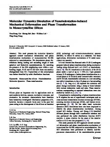
As shown in Fig. 1, the system modeled consisted of a dodecanethiol self-assembled monolayer 共CH3-SAM兲 surface and a nine-residue peptide in explicitly represented physiological saline 共approximately 140 mM NaCl兲. The SAM surface consisted of 90 aliphatic HS– 共CH2兲11 – CH3 chains placed in a 10⫻ 9 array on a 共冑3 ⫻ 冑3兲R30° lattice with a 5.0 Å nearest-neighbor spacing, emulating an alkanethiol layer on the Au 共111兲 plane. Initially, each of the chains was tilted to the orientation described by Vericat et al.,30 although the alkyl portion of the chain is not constrained. In order to preserve the lattice spacing of the SAM chains in the absence of an explicitly represented underlying gold surface, every thiol group 共SH兲 in the SAM was held

87

Yancey et al.: Development of molecular simulation methods

FIG. 1. 共Color online兲 Molecular model of the TGTG-V-GTGT peptide in TIP3P water with approximately 140 mM NaCl over a dodecanethiol SAM surface 关image generated using Visual MD software 共Ref. 34兲 共VMD兲兴. The peptide, the SAM surface, the Na+ 共large yellow兲 and Cl− small 共teal兲 ions in solution, and the fixed layer of water at the top of the unit cell are shown as space-filled atoms. The mobile bulk water molecules are represented by space-filled atoms, which have been made translucent for clarity. The total molecular assembly consists of 12 850 atoms.

fixed during the simulated dynamics. The peptide modeled was chosen to match the experimental methods employed by Wei and Latour,31,32 which had an amino acid sequence of TGTG-V-GTGT 共where T, G, and V represent threonine, glycine, and valine, respectively兲 with zwitterionic end groups. Valine provides hydrophobic character to the peptide in order to enhance its hydrophobic interaction with the methylterminated SAM surface. The flanking repeats of the TG sequence were designed to provide solubility and sufficient molecular weight for detection by surface plasmon resonance spectroscopy.33 During the simulations, interactions between the peptide and the SAM surface were characterized by the surface separation distance 共SSD兲, which is defined as the distance between the average position of the topmost carbon in each SAM chain and the center of mass of the peptide, as illustrated in Fig. 1. To build the mobile solution phase of the system, a TIP3P35,36 water box with the base dimensions of the fixedsulfur lattice in the SAM 共43.3⫻ 45 Å2兲 and an initial height of 35 Å was equilibrated for 500 ps using NPT dynamics at 1 atm and 298 K where only the height of the box was allowed to change. The peptide was placed in the equilibrated water box and all the water molecules whose oxygen resided within a 2.2 Å radius of any peptide atom were deleted. To neutralize the zwitterionic end-groups of the peptide and represent a physiological 140 mM NaCl concentration, a Monte Carlo algorithm was employed to replace 14 randomly chosen TIP3P water molecules with seven sodium ions 共Na+兲 and seven chloride 共Cl−兲 ions. The final number of TIP3P water molecules in the system was 2241. Upon placing the mobile solution phase over the SAM surface, an additional pre-equilibrated 14 Å thick layer of approximately 140 mM saline solution was positioned above the mobile solution with all atoms of this layer fixed in place during simulation. The purpose of this layer was to prevent Biointerphases, Vol. 5, No. 3, September 2010

87

the peptide and saline in the mobile solution phase of the system from interacting with the bottom layer of the SAM surface when using three-dimensional PBCs. When setting up the periodic boundaries in the z direction 共i.e., normal to the surface plane兲, the top of the constrained water layer was fixed 1.2 Å below the bottom of the image SAM surface thiol group. The complete orthorhombic periodic unit cell had base dimensions matching the 43.3⫻ 45 Å2 fixed sulfur lattice in the SAM and a height of 共65.17+ ⌬z兲 Å, where ⌬z is the parameter used to adjust the pressure of the system, which was varied from ⫺2.00 to +2.00 Å in this study. The CHARMM 共Ref. 29兲 simulation program 共version c34b2兲 was used to simulate the dynamics of the model system using CGenFF parameters37 for the SAM and CHARMM22/CMAP parameters16,17 for the peptide and explicit saline solvent. Interactions through periodic boundaries were handled using the CHARMM crystal facility with a sixth-order smooth particle mesh Ewald 共PME兲 summation employed to calculate electrostatic interactions. A spherical Gaussian width of ␬ = 0.34 was used and the PME grid density used 共FFTX = 50, FFTY = 50, and FFTZ = 72兲 was higher than 1 grid point/ Å3. van der Waals interactions were represented using the 12-6 Lennard-Jones potential with a groupbased force-switched cutoff that was invoked at 8 Å and terminated at 12 Å with a nonbonded pair-list generation cutoff at 14 Å. All bonds involving hydrogen atoms were constrained using the RATTLE 共Ref. 38兲 algorithm 关an implementation of SHAKE 共Ref. 39兲 in CHARMM兴, allowing up to a 2 fs time step to be used in the MD simulations. All dynamics were simulated at 298 K under the canonical ensemble 共NVT兲 with a Nosé–Hoover20,40 thermostat in conjunction with the modified velocity Verlet integrator41 共VV2兲. B. Equilibration

Upon its initial assembly, a multistep procedure was used to equilibrate the model system, which we have found to be helpful to minimize the occurrence of SHAKE errors. First, the top methyl and midchain methylene hydrogen atoms of the SAM and the mobile solution phase atoms were relaxed by 100 steps of steepest-descent minimization 共with all other atoms fixed兲 followed by an additional 100 steps where the top methyl carbon atoms of the SAM were also set free to move. The system was then heated from 100 to 298 K with 100 ps of dynamics using a 1 fs time step to relax the SAM’s terminal functional groups on their fixed alkanethiol base. Next, all atoms of the SAM were set free to move except for the thiol base and the system was reheated from 100 to 298 K, followed by an additional 100 ps of dynamics using a 1 fs time step. The system was then equilibrated at 298 K for 400 ps using a 1 fs time step and an additional equilibration was performed for 600 ps using a 2 fs time step where the peptide was harmonically restrained at a SSD of 17 Å to allow the TIP3P water to equilibrate over the SAM surface. The equilibrated system was simulated for an additional 5 ns with the peptide unrestrained using conventional MD with a 2 fs time step. The final structures resulting from these preparation steps were used as the input structures for further sampling to

88

Yancey et al.: Development of molecular simulation methods

determine the pressure and to calculate ⌬Gads. In particular, the data used to calculate the pressure were taken exclusively from an additional 5 ns of conventional MD simulation. For statistical averages of system parameters, three independent simulations were conducted, with different random-number seeds, for each system considered.

88

constant. The instantaneous virial in a bounded system can be calculated as a single sum over the atoms—each having a position vector ri and each being under the influence of a net force Fi, due to all the other atoms in the system: W ⬅ 兺 共ri · Fi兲.

共2兲

i

C. Free energy calculation

To determine the free energy of adsorption, ⌬Gads, a probability ratio method was employed,42 which requires a thorough sampling of the peptide configurations along the entire range of the SSD coordinate. As addressed in our previous work,12,13,18 the configurational sampling obtained by conventional MD is insufficient to calculate ⌬Gads for even simple biomolecular systems 共e.g., a nine-residue peptide兲, requiring the use of advanced sampling techniques such as replica exchange MD 共Ref. 43兲 共REMD兲 to ensure proper coverage of the dihedral space of the peptide. To overcome sampling barriers along the SSD coordinate space, a predetermined biasing potential was applied to the peptide during the REMD simulation of the system, the details of which are published elsewhere.18 For statistical averages, three independent 5 ns biased-REMD simulations were performed for a given system volume using the Multiscale Modeling Tools for Structural Biology44 共MMTSB兲 suite of simulation tools. D. Pressure calculations

Because our model system has fixed atoms, the CHARMM program cannot compute its pressure accurately due to the reasons addressed above. Here we review how pressure is calculated from the internal virial in a conventional MD simulation and introduce a method to calibrate the pressure of a system containing fixed atoms using the pressure of a similar unconstrained system. This calibration is performed by calculating and comparing a local effective virial parameter computed for a cross-sectional layer 共or “slab”兲 of solution in the bulk region of the mobile phase for each system, which is based on the underlying principle that this parameter is directly related to the local pressure of the molecular system. 1. Pressure calculation in a system of unrestrained atoms

1 ¯ ¯ 共2K + W兲. 3V

共1兲

For simulations of N particles in thermal equilibrium having N f degrees of freedom, the equipartition theorem connects the average kinetic energy to the absolute temperature, T, ¯ = 1 N k T, where k is the Boltzmann using the relationship K B 2 f B Biointerphases, Vol. 5, No. 3, September 2010

共rij · fij兲. 兺i 共ri · Fi兲 = 兺i 兺 j⬎i

共3兲

If the system studied is not enclosed by a container but, rather, simulated using PBCs, the pressure relation in Eq. 共1兲 still holds;2,46 however, one must be careful to include the position and influence of the image atoms in the surrounding periodic cells when calculating the virial.47–57 The most common approach for calculating the virial with PBCs is to use the origin-independent pairwise double summation expression indicated on the right-hand-side of Eq. 共3兲, with atom pairs assigned by the minimum image convention.2 Alternatively, if one wishes to use a single-sum virial to evaluate the internal pressure of a periodic system, a computationally inexpensive correction term49 may be added to the virial expressed in Eq. 共2兲. The need for such a correction term when the single summation form of Eq. 共2兲 is used with PBCs can be easily seen if one considers a homogeneous periodic system, such as a simple box of water with surrounding PBCs. In such a case, due to the symmetry of each point in the system, the sum of the force vectors acting on an atom located at any designated position in the system averaged over time will be equal to zero, and thus the time-averaged value of the virial will also be zero irrespective of the system pressure. Alternatively, as is done by the CHARMM program,29 the form of the virial expressed in Eq. 共2兲 may be used without alteration if the image atoms interacting with the primary cell are treated explicitly in terms of accounting for their positions and force contributions from the atoms in the primary simulation cell. This can be expressed by N

When enclosed in a volume, V, a molecular system in mechanical equilibrium exerts a uniform pressure, P, on the boundaries of its container that can be calculated from the virial theorem of Clausius2,45 in terms of the time-averaged ¯ , of the molecules and the time-averaged kinetic energy, K ¯: virial, W P=

When the net force acting on each atom can be expressed as a superposition of pairwise forces 共i.e., Fi = 兺 j⫽ifij over interatomic distances, rij ⬅ ri − r j兲, the single-sum virial is often rewritten as a pairwise sum using2,45

W = 兺 共ri · Fi兲 + i=1

MN

兺 共ri · Fi⬘兲, i=N+1

共4兲

where N represents the number of atoms contained in the primary cell of the system, M represents the number of periodic image cells surrounding the primary cell, Fi represents the sum of the force vectors from all atoms 共i.e., primary and image atoms兲 acting on atom i within the primary cell, and Fi⬘ represents the sum of the force vectors from the atoms in the primary cell acting on an image atom i, without including the force contributions from the other image atoms. Equation 共4兲 is identical to the relationship developed by Thompson et al.49 to provide the correction necessary for the use of the single summation method for the calculation of pressure when using PBCs, and it can be readily shown that the rela-

89

Yancey et al.: Development of molecular simulation methods

tionship expressed in Eq. 共4兲 is equivalent to the double sum expression shown on the right-hand-side of Eq. 共3兲. 2. Pressure calculation for a system having fixed atoms

It is often expedient to fix the positions of atoms in a molecular dynamics simulation; however, the use of rigid constraints 共which are external, nonconservative forces兲 make nonphysical contributions to the system virial, and thus may adversely affect the pressure represented by Eq. 共1兲.58 To address this problem, the pairwise-sum virial determined by Eq. 共3兲 can be partitioned into a sum of three pair-type contributions: W = W f f + Wmm + W fm ,

共5兲

where W f f is the contribution to the virial from pairs of fixed atoms, Wmm is the contribution from pairs of mobile atoms, and W fm is of the contribution from forces between fixed and mobile atoms. As Smith and Rodger58 pointed out, the W f f term is based on fixed positions only and does not scale with the system volume. Since pressure is determined by the scaling of the free energy with volume according to the thermodynamic relationship, P=−

冉 冊 ⳵A ⳵V

,

共6兲

T

it is clear that W f f should not be considered when calculating the system pressure and should be set to zero 关although codes such as NAMD 共Ref. 59兲 give the user the option of including these forces with the admonition that the interactions between constrained atoms be minimized prior to fixing them兴. The Wmm and W fm terms are readily computed as pairwise-sum virials. However, even if the forces of constraint acting on fixed atoms are properly handled in computing the virial, and the number of the degrees of freedom in the system 共N f 兲 is adjusted accordingly to determine the kinetic energy, the presence of fixed atoms can still cause problems by making it difficult to accurately define the volume of the system that is accessible to the mobile atoms, thus further complicating the accurate calculation of the system pressure. Using an argument with atoms approximated by hard spheres, Smith and Rodger58 showed that the W fm term is responsible for a reduction in system volume due to the fixed atoms; however, it is often very difficult to determine how this term influences the total volume in cases where the fixed atoms enclose some excluded volume that is inaccessible to the mobile atoms. Moreover, the use of atomic constraints impedes the implementation of fractional coordinate scaling methods that are used to optimize and maintain system pressure in common constant pressure-temperature 共CPT兲 dynamics algorithms. This restriction may necessitate MD simulations with fixed atoms to be simulated in the NVT ensemble, thus requiring that the overall system volume be set to a user-defined value. For example, some simulation programs, such as CHARMM, do not allow one to invoke CPT dynamics when atomic constraints are in use, while other programs, such as AMBER 共Ref. 60兲 and NAMD,59 allow fixed Biointerphases, Vol. 5, No. 3, September 2010

89

atoms to be used with CPT dynamics while warning not to use a significant number of them. Accordingly, it should be understood that the internal pressure reported by standard MD programs for a system containing fixed atoms might not accurately represent the pressure of the system. One way around the problems caused by fixed atoms is to calculate the local pressure using a small defined volume of fully mobile atoms within the larger system that is at least a cutoff distance removed from any of the fixed atoms in the system, thus minimizing their influence on the local pressure of the system. This can be done using local pressure tensor methods27,28 or by using a virial-based approach. For a simulation program that utilizes a pairwise virial formulation for the pressure, the local pressure of a small volume segment of the system 共denoted a slab, although it could have any geometry兲 could be determined from a virial such as slab slab

slab outside

Wslab = 兺 兺 共rij · fij兲 + 兺 i

j⬎i

i

兺 j⬎i

共rij · fij兲,

共7兲

where slab and “outside” refer to atoms inside and outside of the defined local volume within the primary cell, respectively, with the corresponding volume and kinetic energy of the atoms contained within the slab used for the calculation of the pressure using Eq. 共1兲. Equation 共7兲 is analogous to the form of the virial used to calculate the pressure for an unconstrained system with PBCs with the slab representing the primary cell and the volume outside the primary cell slab representing the surrounding periodic images. It is important to again note that when using PBCs, the pressure in the slab can be appropriately calculated using the summation over the relative position and force vectors 共i.e., rij and fij, respectively兲, but not from the summation over the individual position and total force vectors 共i.e., ri and Fi, respectively兲 for the atoms within the slab alone.2,45 This can be readily shown by the fact that for a general slab volume within a larger molecular system: slab all

slab

共rij · fij兲 ⫽ 兺 共ri · Fi兲. 兺i 兺 j⬎i i

共8兲

关The inequality of Eq. 共8兲 can be demonstrated with a simple three-atom system in which two of the atoms are placed within a slab and one atom is placed outside of the slab.兴 In order to use the single summation form of the virial for a local slab, the positions and force contributions between the slab atoms and the atoms outside the slab must be taken into consideration in a manner similar to the treatment of the image atoms for the application of the single-sum virial shown in Eq. 共4兲. This relationship can be expressed as S

Wslab = 兺 共ri · Fi兲 + i=1

N

兺

i=S+1

共ri · Fi⬘兲 +

兺

共ri · Fi⬙兲,

共9兲

image

where atoms i = 1 to S and i = S + 1 to N represent the atoms inside and outside the local slab within the primary cell, “image” refers to the atoms in the surrounding periodic images of the primary cell, Fi⬘ represent the force vectors due to atoms within the slab acting upon atoms outside of the

90

Yancey et al.: Development of molecular simulation methods

slab within the primary cell, and Fi⬙ represent the force vectors from the slab atoms within the primary cell acting on the image atoms. Unfortunately, programs that use a single-sum pressure evaluation in a manner that appropriately considers the positions and force contributions of the image atoms for the calculation of pressure for the whole molecular system, like that expressed in Eq. 共4兲 共e.g., CHARMM兲, are typically not designed to calculate the internal virial for a local volume of the system. While such programs can easily be adapted to account for the contributions of the first term on the righthand-side of Eq. 共9兲, representation of the second and third terms generally would require substantial code modification. As an alternative, however, single-sum virial calculation methods can be readily adapted to calculate what we refer to as an effective virial, We, which is still directly related to the local pressure. We define this effective virial as S

We = 兺 共ri · Fi兲 + i=1

兺

共ri · Fi⵮兲,

共10兲

slab image

where the first term on the right-hand-side is the same as the first term in Eq. 共9兲, while ri in the second term represents the positions of the atoms in the images of the slab and Fi⵮ represents the force vectors from primary cell atoms 共both inside and outside of the slab兲 acting on the atoms lying within the images of the slab. We then also define a parameter that represents the effective virial per atom as we共 =We / Ns兲, where Ns is the number of atoms contained within the defined slab volume. In the case of a system composed of a mobile solution phase over a solid phase containing fixed atoms, we can be calculated for a defined slab volume within the mobile solution phase that is free of the influence of system constraints. It could then be used to determine the actual internal pressure of the solution phase of the system if a calibration plot between the value of this effective virial and internal pressure could be provided. This calibration plot can be simply generated by setting up a simulation system representing a box of plain solvent without any atomic constraints applied with equivalent cross-sectional dimensions, total number of solvent atoms, and similar solvent box height as the one used for the mobile solution in the simulation with fixed atoms 共i.e., mobile solution shown in Fig. 1兲. The effective virial per atom 共we兲 can then be calculated for a slab of solvent in the plain solvent system that has equivalent dimensions as in the system with fixed atoms, with the height of the overall plain solvent box varied while keeping the number of solvent atoms constant, thus varying its pressure. In this case, because no atoms are constrained, the system pressure can be accurately calculated along with we of the defined slab during the simulation. The values of we under these different pressure conditions can then be plotted against the accurately computed pressure to obtain a calibration plot for the we parameter. Then, returning to the system with fixed atoms, we of the solvent slab of the mobile solvent atoms can be calculated for the same-dimensioned slab as with the unconstrained plain solvent box. The pressure calibration plot can Biointerphases, Vol. 5, No. 3, September 2010

90

then be used to determine the pressure in the solution phase of this system from the corresponding we values, with the height of the solvent box in the system with atomic constraints then adjusted as necessary until the desired solution pressure is obtained. To demonstrate this approach, we defined a crosssectional layer of solvent within the solution phase of our peptide-SAM model system as the slab. This slab had a height of 5 Å and a base identical to the 43.3⫻ 45 Å2 base of the primary simulation cell 共see Fig. 1兲. The position of the slab was chosen so that the pressure of the solvent in the SSD region from 15–20 Å could be monitored, placing its bottom more than a cutoff radius away from the SAM surface and its top more than a cutoff radius away from the bottom of the fixed water layer. The plain solvent system 共i.e., system without constraints兲, which was used for generating the we versus P calibration plot, was created by placing an exact replica of the mobile solution phase of the peptideSAM model system 共i.e., all the TIP3P waters, ions, and the peptide兲 in a 43.3⫻ 45⫻ 35 Å3 box with periodic boundary conditions. This solvent box was then simulated under NVT conditions for overall box heights ranging from 32 to 38 Å to obtain values of we over a wide range of pressures. When calculating we, the net force acting on each atom present in the slab included all bonded interactions 共corrected for 41 SHAKE/RATTLE when appropriate 兲 and nonbonded interactions with neighboring atoms within the 12 Å cutoff 共both primary and image兲 as well as the forces due to the longrange PME electrostatic interactions. Once the calibration plot is generated, it can be used to determine the value of we that corresponds to any desired pressure 共e.g., 1 atm兲. The height of the solvent box of the peptide-SAM system with the constrained atoms can then be adjusted until the value of we for the equivalent slab in the peptide-SAM system matches the designated value from the calibration plot, thus establishing conditions representing the desired solution pressure for the simulation of peptide adsorption behavior.

III. RESULTS AND DISCUSSION Before addressing the influence of pressure on the values of ⌬Gads for peptide adsorption to the SAM surface, we first present our results for applying the developed approach to accurately determine the pressure of the peptide solution over the SAM surface despite the use of constraints to lock the positions of portions of the system. These results show that the default pressure value reported in CHARMM for this system is in error by several hundred atmospheres, with the correct solution pressure being able to be determined using the effective virial. We then apply this method to quantitatively show that pressure does indeed have a significant effect on ⌬Gads, thus demonstrating the importance of correctly determining and controlling pressure for the accurate simulation of peptide or protein adsorption behavior. Supporting analyses are also provided to address the physical changes at the interphase that lead to the relationship between ⌬Gads and pressure, which we relate to the influence

91

Yancey et al.: Development of molecular simulation methods

FIG. 2. 共Color online兲 Two-stage pressure optimization process: 共a兲 Calibration plot showing the relationship between the internal pressure and the effective virial per atom 共we兲 for a 5 Å thick cross-sectional slab of the plain solvent box without atom constraints 共black squares; linear regression equation and R2 correlation coefficient兲. For comparison, the CHARMM reported internal pressure for the system with atomic constraints 共i.e., peptide over SAM surface兲 is also shown 共blue triangles兲. 共b兲 Relationship between effective virial parameter we and changes in solvent box height for the peptide-SAM system with constrained atoms. Conditions providing 1 atm pressure for the constrained system are provided by adjusting the height 共⌬z兲 of the solvent box in the constrained system to provide a value of we that is equivalent to the 1 atm condition for the plain solvent box system. Error bars represent ⫾95% CIs obtained from three independent simulations. 95% CI values for the water box pressure data points in 共a兲 are less than 40 atm and are around 100 atm for the system with fixed atoms.

of pressure on the structure of TIP3P water over the hydrophobic SAM surface. A. Pressure calibration

The plot showing the relationship between system pressure and the mean we obtained from three independent 5 ns conventional MD simulations of the solvent slab in the plain solvent box without any constraints is presented in Fig. 2共a兲. For statistical averages, a single 5 ns time-averaged we was taken from each of three independent conventional MD simulations and averaged together to yield an estimate of the mean of the data and 95% CIs about the mean. Corresponding pressures for each of the three simulations were quite reproducible, with 95% confidence intervals typically being less than 40 atm. As shown in this figure, a very strong linear correspondence clearly exists between we and system pressure with an R2 correlation coefficient of 0.9969. We should also note here that the “negative” pressures, which commonly occur in condensed-phase simulations, indicate a situation where the system has been metastably overexpanded, but not to the point of cavitating to form a bubble of vapor phase. In addition to the results presented in Fig. 2共a兲, we of the plain solvent system was also calculated in preliminary Biointerphases, Vol. 5, No. 3, September 2010

91

studies for slabs of thickness varying from 5 to 15 Å to check for nonphysical artifacts due to slab size. The results from these studies showed that we was constant irrespective of slab thickness, confirming the robustness of this parameter. In addition, to determine if we was significantly affected by the presence of the mobile peptide during these simulations, the solvent box was simulated both with and without the peptide, and the resulting we values were indistinguishable from one another. Figure 2共b兲 presents the relationship between the change in total height of the solvation box 共i.e., ⌬z兲 and the calculated value of we for the system with constrained atoms. The height of the model system was varied over a 4 Å range about the nominal total system height of 65.17 Å and the resulting data were fitted with a smooth Bezier curve of degree 9. As shown in Fig. 2, the value of we corresponding to a pressure of about 1 atm in the plain solvent box 共−0.778 kcal mol−1 atom−1兲 indicates that the height adjustment required to provide 1 atm pressure conditions for the solution phase in the peptide-SAM system was ⫺0.38 Å. Figure 2共a兲 also shows the internal pressure for the whole system reported directly by CHARMM for the peptide-SAM system with the constrained atoms. For the we value that corresponds to a pressure of 1 atm in the system with atom constraints, CHARMM reports a pressure above 500 atm, thus demonstrating the substantial amount of error that can be present in the default calculation of pressure for systems with constrained atoms. Using the previously mentioned compressibility of water at 298 K and 1 atm, a difference in 500 atm in pressure corresponds to an error on the order of 2% in the solvent box volume or difference in height of about 1.5 Å for the system shown in Fig. 1. This value is consistent with the difference in ⌬z values needed to cause a change in solvent box pressures from 1 and 500 atm in Fig. 2. As a further check on the relationship between the ⌬z values and the estimated pressure of the solvent, an additional system was simulated with a 20 Å layer of vacuum positioned over the mobile phase of water in the system 共i.e., greater than the cutoff distance兲, so that the pressure in this system would be the vapor pressure of water at 298 K, which lies close to zero pressure. The slab in this vapor/liquid system had an average we of −0.781⫾ 0.006 kcal mol−1 atom−1 共mean ⫾95% confidence interval兲, which corresponds to an average pressure of −9.4⫾ 22 atm. This is statistically indistinguishable from the expected zero pressure, again supporting the validity of the developed approach. The number of samples chosen to create the calibration plot in Fig. 2 was qualitatively based on the initial dimensions of the system. To generate such a plot for a general system with constraints it is recommended that a slab be chosen with a shape to meet the characteristic geometry of the system considered with the caveat that the slab be present in the bulk of the mobile solvent of the system, separated by more than a cutoff radius from any constrained atoms at all times. An NPT simulation for a large unconstrained box of the solvent found in this system should be equilibrated at the desired pressure 共in our case 1 atm兲 and the mean volume

92

Yancey et al.: Development of molecular simulation methods

FIG. 3. 共Color online兲 Cumulative average of the effective virial per atom parameter 共we兲 for the 5 Å thick slab as a function of conventional MD simulation time beyond equilibration for three independent simulations 共three simulations initialized with distinct random number seeds during heating兲 of a system with ⌬z = −0.40 Å. The illustrated stabilization of we is typical for all of the systems shown in Fig. 2, indicating that at least 2–3 ns of dynamics are required for the creation of a reliable calibration plot.

corresponding to this pressure can then be used as the central point for the volume to be used in generating the calibration plot. Subsequent NVT simulations can then be conducted in ⫾1% increments of increased volume over a range of ⫾0%– 5%, which should roughly correspond to ⫾1000 atm based on the compressibility of water at 298 K. A plot similar to Fig. 3 can be used to determine the appropriate amount of time needed to sample the pressure of an equilibrated model system. The cumulative average of we for the slab modeled in this article was typically found to stabilize for a given SAM-peptide system after 2–3 ns of conventional MD. Running multiple independent simulations 共three or more兲 that have been initialized with distinct random number seeds is needed to describe the statistical behavior of the mean we and thus the pressure. Although we are not able to provide a clear proof that the relationship between P and we must be the same in the constrained system as in the unconstrained system, the fact that we is dominated by pairwise interatomic forces that are represented within the cutoff distance of atoms that interact with the atoms within the defined slab volume, and the fact that the unconstrained and constrained molecular systems are essentially identical to one another 共apart any significant contribution from long-range electrostatics in the system兲 within this region of each system, leads to the logical conclusion that the relationship between P and we should be identical in both systems. This conclusion is supported by the vacuum layer system, which imposes a known pressure between 0⫺1 atm, with the corresponding we value for the slab atoms in this constrained system being in excellent agreement with the P versus we calibration plot obtained from the unconstrained system. B. Effect of pressure on ⌬Gads

Given the ability to accurately determine the solution pressure in our peptide-SAM system, we were able to directly evaluate its effect on peptide adsorption behavior. The Biointerphases, Vol. 5, No. 3, September 2010

92

FIG. 4. 共Color online兲 Effect of pressure on the free energy profile for peptide adsorption to a CH3-SAM surface. The PMFs shown were extracted from biased-REMD simulations of the peptide-SAM model systems for relative heights of ⌬z = −2.00 Å 共high pressure; about 710 atm兲, ⫺0.73 Å 共moderate pressure; about 100 atm兲, and +1.50 Å 共low pressure; about ⫺510 atm兲. Error bars represent 95% CI values obtained from three independent simulations.

effect of pressure on the free energy of peptide adsorption is illustrated for three systems in Fig. 4, including one with a relative height of ⌬z = −2.00 Å 共high pressure; about 720 atm兲, one with ⌬z = +1.50 Å 共low pressure; about ⫺540 atm兲, and ⌬z = −0.73 Å 共moderate pressure; about 100 atm兲. To obtain the PMF profile shown for each system, biasedREMD simulations using 24 exponentially spaced replicas from 298 to 400 K were performed with 5 ns of production sampling. The configurational ensembles, which were analyzed to calculate ⌬Gads using the probability ratio method,18,42 were obtained from the 298 K replicas. Based on the free energy profiles along the SSD coordinate at various pressures shown in Fig. 4 and the resulting values of ⌬Gads, which are presented in Table I, solution pressure is shown to have a large effect on peptide adsorption behavior with substantially weaker adsorption occurring in high pressure systems compared to systems at low pressure. This is clearly visible from the shallower PMFs at high pressure in Fig. 4, as well as the calculated ⌬Gads values in Table I. The adsorption free energy of ⫺1.88 kcal/mol at moderate pressure is decreased by over 80% when the pressure is elevated by ⬃620 atm, and is strengthened by nearly 40% when the pressure is reduced by ⬃640 atm. These results indicate that it is extremely important for a simulation of peptide 共or protein兲 adsorption to have the pressure set correctly during a MD simulation, which can be accomTABLE I. Free energy of adsorption extracted from the PMF profiles in Fig. 4. The error bars reported are 95% confidence intervals obtained from three independent 5 ns biased-REMD simulations. ⌬z 共Å兲

P 共atm兲

⌬Gads 共kcal/mol兲

⫺2.00 ⫺0.73 1.50

720⫾ 58 100⫾ 80 −540⫾ 180

−0.34⫾ 0.42 −1.88⫾ 0.93 −2.60⫾ 0.47

93

Yancey et al.: Development of molecular simulation methods

93

TABLE II. Pressures obtained for various relative system heights 共⌬z兲. The error bars reported are 95% confidence intervals obtained from three independent 5 ns conventional MD simulations. ⌬z 共Å兲 ⫺2.00 ⫺1.50 ⫺1.00 ⫺0.50 ⫺0.45 ⫺0.40 ⫺0.35 ⫺0.30 0.00 0.50 1.00 1.50 2.00 Vacuum

FIG. 5. 共Color online兲 Atomic density distribution, ␳, of the TIP3P solvent as a function of z, the distance from the plane of the CH3-SAM surface, for 共a兲 the full range of relative system heights, ⌬z, and 共b兲 a small subset of relative heights that closely match the “Vacuum” system density. The trend labeled “Vacuum” shows the water structure for a system modeled with a 20 Å layer of vacuum placed over the mobile solution phase, thus imposing conditions representing a pressure near 0 atm 共−9.4⫾ 22 atm per Fig. 2兲.

plished by adjusting the height of the solvent box in the system to match a corresponding value of we using the calibration methods outlined above. Naively trusting the reported pressure in a system with constrained atoms can lead to large pressure errors, and thus to substantial errors in adsorption energy. In the 12 850 atom system simulated, 2680 of the atoms were fixed 共roughly 20%兲 and the error in the CHARMM reported pressure was on the order of 500 atm 共Fig. 2兲. C. Interfacial pressure effects

To provide some understanding of the physical effects that lead to the variability of ⌬Gads with pressure, water structure profiles over the SAM surface were examined over a range of pressures induced by imposing different values of ⌬z. The density of the water over the SAM surface under these various pressures is illustrated in Fig. 5 by the z-coordinate distribution function 共ZDF兲 共i.e., the number density ␳共z兲 of water molecules along the z axis perpendicular to the surface plane兲 as a function of the z-coordinate position relative to the SAM surface. The ZDF data shown Biointerphases, Vol. 5, No. 3, September 2010

P 共atm兲 720⫾ 58 480⫾ 47 240⫾ 29 30⫾ 71 19⫾ 38 −21⫾ 20 −31⫾ 55 −71⫾ 55 −120⫾ 110 −360⫾ 49 −480⫾ 110 −540⫾ 180 −560⫾ 78 −9.4⫾ 22

are averages taken from 10 ns of conventional MD under the canonical ensemble 共i.e., NVT conditions兲 performed on the equilibrated system and, for every relative height ⌬z shown, pressures measured from the calibration plot 共Fig. 2兲 are reported in Table II with 95% CI obtained from three independent simulations. The general features of these ZDFs are in agreement with previous simulations4,61 and experimental results.61,62 At the highest pressure simulated 共⌬z = −2.00 Å; P = 720 atm兲, the ZDF shows a strongly ordered solvent at the interface, with at least two distinct peaks near the SAM surface—one near z = 3.30 Å and one near z = 6.30 Å. As the relative system height, ⌬z, is increased, the internal pressure of the system decreases and the solvent becomes less structured and less dense at the interface. This change in water density near the SAM surface is proposed to be responsible for the substantial effect of pressure on peptide adsorption free energy, with the peptide having to displace an increasingly higher density of close-packed water at the surface as the pressure increases, thus providing increased resistance to adsorption to the SAM surface. The green ZDF trend, labeled “Vacuum,” representing conditions of −9.4⫾ 22 atm, was obtained from the simulation under the liquid/vapor equilibrium, and has solvent layer peaks near z = 3.41 Å and z = 6.49 Å. This plot follows the trend of the ⌬z = −0.50 Å relative height more closely than any other systems modeled in Fig. 5共a兲. When plotted on a finer scale that focuses on the first solvation peak 关Fig. 5共b兲兴, the green Vacuum ZDF trend lies between the ⌬z = −0.40 Å and ⌬z = −0.45 Å trends, which agrees well with the ⌬z = −0.38 Å obtained from the calibration plot 共Fig. 2兲, thus independently confirming the accuracy of the pressure optimization technique. Images of the water structure for the highest and lowest pressure systems are shown in Figs. 6共a兲 and 6共b兲, respectively. These images clearly illustrate how pressure influences water structure and density at the interphase region of the system, and it

94

Yancey et al.: Development of molecular simulation methods

FIG. 6. 共Color online兲 Structuring of water layers over the CH3-SAM in a conventional MD simulation by CHARMM 关illustrated by VMD 共Ref. 34兲兴 when the system is under 共a兲 high pressure conditions, seen when ⌬z = −2.00 Å 共P = 720 atm兲, and 共b兲 low pressure conditions, seen when ⌬z = +2.00 Å 共P = −560 atm兲.

is not surprising that these dramatic changes to water structure would have a strong influence on peptide adsorption behavior. IV. CONCLUSIONS AND FUTURE DIRECTIONS When simulating peptide or protein adsorption to a solidphase surface, it is often necessary to lock atoms in place using fixed constraints to ensure proper positioning of surface substrate lattices and/or to reduce the computational cost of the simulation. The use of constraints, however, imposes nonconservative external forces on the system and causes difficulties in defining the volume occupied by the unconstrained atoms in the system, both of which can substantially affect the ability to accurately calculate the internal pressure. This, plus an inability to use fractional coordinate scaling to control the system volume, interferes with the ability to perform simulations under constant pressure conditions. These factors are of particular concern in the simulation of peptide and protein adsorption behavior because, as we have shown in this study, the strength of adsorption of a peptide on a surface can be substantially influenced by the pressure of the system. To address these problems, we have developed and demonstrated a relatively simple method to accurately determine the pressure of a molecular system that contains constrained atoms by calculating an effective virial parameter, we, for a local region of the system containing only mobile atoms and calibrating this effective virial against a plain solvent system without atom constraints, for which the pressure can be accurately determined using the standard virial method. This approach allows the volume of the mobile solution phase of a molecular system containing fixed atoms to be adjusted so that the local effective virial corresponds to the desired pressure of the system, enabling simulations of peptide or protein adsorption to be conducted at the appropriate pressure. Although the methods presented in this article were conducted under NVT conditions in which the volume of the mobile solution phase of the system was manually adjusted in order to achieve the desired pressure, a similar approach could easily be implemented in an automated fashion. In such a case, the value of we could be monitored during a MD simulation and the height of the solvent box could be adjusted to maintain a targeted average value of this parameter. Biointerphases, Vol. 5, No. 3, September 2010

94

This type of simulation, which may be referred to as NweT conditions, may be particularly important when conducting a simulation that involves adsorption-induced unfolding of a protein. In this case, the change in the molecular volume of the protein that may occur as a result of unfolding can be expected to substantially alter the pressure of the solution phase of the system if the simulation were conducted under NVT conditions,63 with subsequent nonphysical artifacts introduced in the adsorption behavior of the protein due to the changes in solution pressure. However, by monitoring we and adjusting the height of the solvent box to maintain it within a targeted range, the solution pressure can be maintained at the target value, thus enabling the system to be simulated under constant solution pressure conditions as necessary for the accurate simulation of protein adsorption behavior. ACKNOWLEDGMENTS This work was funded under NIH Grant No. R01 EB006163. Partial support was also provided by “RESBIOThe National Resource for Polymeric Biomaterials” funded under NIH Grant No. P41 EB001046 and NIH Grant No. R01 GM074511. The authors thank J. Barr von Oehsen and Corey Ferrier for support of the Palmetto Cluster computational resources at Clemson University. 1

A. R. Leach, Molecular Modelling: Principles and Applications, 2nd ed. 共Pearson Education, Harlow, UK, 2001兲, pp. 165–170 and 303–351. 2 M. P. Allen and D. J. Tildesley, Computer Simulation of Liquids 共Oxford University Press, Oxford, UK, 1987兲, pp. 1–32 and 46–49. 3 A. J. Pertsin and M. Grunze, Langmuir 16, 8829 共2000兲. 4 A. J. Pertsin, T. Hayashi, and M. Grunze, J. Phys. Chem. B 106, 12274 共2002兲. 5 Y. Sun and R. A. Latour, J. Comput. Chem. 27, 1908 共2006兲. 6 R. A. Latour, Curr. Opin. Solid State Mater. Sci. 4, 413 共1999兲. 7 G. E. Wnek and G. L. Bowlin, Encyclopedia of Biomaterials and Biomedical Engineering, 2nd ed. 共Informa Healthcare, New York, 2008兲, Vol. 1, pp. 270–284. 8 K. Wilson, S. J. Stuart, A. Garcia, and R. A. Latour, J. Biomed. Mater. Res. Part A 69A, 686 共2004兲. 9 M. Agashe, V. Raut, S. J. Stuart, and R. A. Latour, Langmuir 21, 1103 共2005兲. 10 R. A. Latour and L. L. Hench, Biomaterials 23, 4633 共2002兲. 11 C. E. Nordgren, D. J. Tobias, M. L. Klein, and J. K. Blasie, Biophys. J. 83, 2906 共2002兲. 12 F. Wang, S. J. Stuart, and R. A. Latour, BioInterphases 3, 9 共2008兲. 13 C. P. O’Brien, S. J. Stuart, D. A. Bruce, and R. A. Latour, Langmuir 24, 14115 共2008兲. 14 G. Collier, N. A. Vellore, R. A. Latour, and S. J. Stuart, BioInterphases 4, 57 共2009兲. 15 X. F. Li, C. P. O’Brien, G. Collier, N. A. Vellore, F. Wang, R. A. Latour, D. A. Bruce, and S. J. Stuart, J. Chem. Phys. 127, 164116 共2007兲. 16 A. D. MacKerell et al., J. Phys. Chem. B 102, 3586 共1998兲. 17 A. D. Mackerell, M. Feig, and C. L. Brooks, J. Comput. Chem. 25, 1400 共2004兲. 18 N. A. Vellore, J. A. Yancey, G. Collier, R. A. Latour, and S. J. Stuart, Langmuir 26, 7396 共2010兲. 19 H. C. Andersen, J. Chem. Phys. 72, 2384 共1980兲. 20 S. Nosé and M. L. Klein, Mol. Phys. 50, 1055 共1983兲. 21 P. V. Hobbs, Ice Physics 共Clarendon, Oxford, UK, 1974兲, pp. 346–348. 22 G. Hummer, S. Garde, A. E. Garcia, M. E. Paulaitis, and L. R. Pratt, Proc. Natl. Acad. Sci. U.S.A. 95, 1552 共1998兲. 23 S. W. Rick, J. Phys. Chem. B 104, 6884 共2000兲. 24 T. Ghosh, A. E. Garcia, and S. Garde, J. Am. Chem. Soc. 123, 10997 共2001兲. 25 Y. Sun, B. N. Dominy, and R. A. Latour, J. Comput. Chem. 28, 1883 共2007兲.

95

Yancey et al.: Development of molecular simulation methods

A. Wallqvist, J. Chem. Phys. 96, 1655 共1992兲. H. Heinz, W. Paul, and K. Binder, Phys. Rev. E 72, 066704 共2005兲. 28 H. Heinz, Mol. Simul. 33, 747 共2007兲. 29 B. R. Brooks et al., J. Comput. Chem. 30, 1545 共2009兲. 30 C. Vericat, M. E. Vela, G. A. Benitez, J. A. M. Gago, X. Torrelles, and R. C. Salvarezza, J. Phys.: Condens. Matter 18, R867 共2006兲. 31 Y. Wei and R. A. Latour, Langmuir 24, 6721 共2008兲. 32 Y. Wei and R. Latour, Langmuir 25, 5637 共2009兲. 33 R. J. Green, R. A. Frazier, K. M. Shakesheff, M. C. Davies, C. J. Roberts, and S. J. B. Tendler, Biomaterials 21, 1823 共2000兲. 34 W. Humphrey, A. Dalke, and K. Schulten, J. Mol. Graphics 14, 33 共1996兲. 35 W. L. Jorgensen, J. Chem. Phys. 77, 4156 共1982兲. 36 W. L. Jorgensen, J. Chandrasekhar, J. D. Madura, R. W. Impey, and M. L. Klein, J. Chem. Phys. 79, 926 共1983兲. 37 K. Vanommeslaeghe et al., J. Comput. Chem. 31, 671 共2010兲. 38 H. C. Andersen, J. Comput. Phys. 52, 24 共1983兲. 39 J. P. Ryckaert, G. Ciccotti, and H. J. C. Berendsen, J. Comput. Phys. 23, 327 共1977兲. 40 S. Nosé, Mol. Phys. 52, 255 共1984兲. 41 G. J. Martyna, M. E. Tuckerman, D. J. Tobias, and M. L. Klein, Mol. Phys. 87, 1117 共1996兲. 42 M. Mezei and D. Beveridge, Ann. N.Y. Acad. Sci. 482, 1 共1986兲. 43 Y. Sugita and Y. Okamoto, Chem. Phys. Lett. 314, 141 共1999兲. 44 M. Feig, J. Karanicolas, and C. L. Brooks, J. Mol. Graphics Modell. 22, 377 共2004兲. 45 G. Marc and W. G. McMillan, Adv. Chem. Phys. 58, 209 共1985兲. 26 27

Biointerphases, Vol. 5, No. 3, September 2010

46

95

J. J. Erpenbeck and W. W. Wood, in Statistical Mechanics B: Modern Theoretical Chemistry, edited by B. J. Berne 共Plenum, New York, 1977兲, Vol. 6, pp. 1–41. 47 D. Brown and S. Neyertz, Mol. Phys. 84, 577 共1995兲. 48 M. J. Louwerse and E. J. Baerends, Chem. Phys. Lett. 421, 138 共2006兲. 49 A. P. Thompson, S. J. Plimpton, and W. Mattson, J. Chem. Phys. 131, 154107 共2009兲. 50 H. Bekker, E. J. Dijkstra, M. K. R. Renardus, and H. J. C. Berendsen, Mol. Simul. 14, 137 共1995兲. 51 P. H. Hünenberger, J. Chem. Phys. 116, 6880 共2002兲. 52 B. Oliva and P. H. Hunenberger, J. Chem. Phys. 116, 6898 共2002兲. 53 R. G. Winkler, H. Morawitz, and D. Y. Yoon, Mol. Phys. 75, 669 共1992兲. 54 R. G. Winkler and R. Hentschke, J. Chem. Phys. 99, 5405 共1993兲. 55 R. G. Winkler, J. Chem. Phys. 117, 2449 共2002兲. 56 R. L. C. Akkermans and G. Ciccotti, J. Phys. Chem. B 108, 6866 共2004兲. 57 D. H. Tsai, J. Chem. Phys. 70, 1375 共1979兲. 58 W. Smith and P. M. Rodger, The pressure in systems with frozen atoms, in Collaborative Computational Projects 5 共CCP5兲 共2002兲, see http:// www.ccp5.ac.uk/infoweb/wsmith22/wsmith22.pdf. 59 J. C. Phillips et al., J. Comput. Chem. 26, 1781 共2005兲. 60 D. A. Case et al., J. Comput. Chem. 26, 1668 共2005兲. 61 R. R. Netz, Curr. Opin. Colloid Interface Sci. 9, 192 共2004兲. 62 D. Schwendel, T. Hayashi, R. Dahint, A. Pertsin, M. Grunze, R. Steitz, and F. Schreiber, Langmuir 19, 2284 共2003兲. 63 E. Paci, Biochim. et Biophys. Acta 共BBA兲–Protein Struct. Mol. Enzymol. 1595, 185 共2002兲.