Development of q-exponential models for tree height, volume and

International Journal of the Physical Sciences Vol. 5(15), pp. 2369-2378, 18 November, 2010 Available online at http://www.academicjournals.org/IJPS ISSN 1992 - 1950 ©2010 Academic Journals

Full Length Research Paper

Development of q-exponential models for tree height, volume and stem profile Petras Rupšys1,2* and Edmundas Petrauskas1 1

Department of Forest Management, Lithuanian University of Agriculture, Studentu 11, Akademija, Kauno distr. 53361, Lithuania. 2 Department of Mathematics, Lithuanian University of Agriculture, Studentu 11, Akademija, Kauno distr. 53361, Lithuania. Accepted 29 October, 2010

New models for tree height stem volume and taper (stem profile) were developed using a q-exponential function in the symbolic computational language MAPLE. Three previously constructed models and a new q-exponential model for height stem volume and taper were employed to compare predicted values with empirical values of height, stem volume and diameter outside bark. Performance statistics for the height stem volume and taper equations included four statistical indices: mean bias, mean absolute bias, mean percentage of absolute bias, and a coefficient of determination. A stem analysis of 1925 Scots pine (Pinus sylvestris) trees provided the data for this study. The new q-exponential models were superior to the previously constructed models in predicting height, stem volume and taper. Key words: Stem taper model, q-exponential function, tree allometry, Scots pine. INTRODUCTION Complex inventories of forests require accurate estimates of the total and merchantable volume of each tree. For several decades, forest science focused much attention on modelling individual tree height, taper and volume as functions of individual tree attributes. Traditionally, relationships between predictor variables and tree biomass, height, taper and volume have been described based on regression models (Salazar et al., 2008; Zianis et al., 2005). Height-diameter relationships are used to estimate the heights of trees based solely on data for diameter at breast height. In most sample plot systems (Marshall et al., 2000), diameter at breast height conventionally is measured for all trees sampled, whereas height is measured only for a sub-sample. Consequently, the height-diameter regression model affects estimates of individual tree volume. To improve inventory efficiency, merchantable tree height and both total and merchantable tree stem volume can be estimated using tree taper models (Max and Burkhart,

*Corresponding author. E-mail: [email protected]. Tel/Fax: +370 37 752269/+370 37 752379.

1976). Taper functions can become the primary tool for estimating the volume at any part of the trunk, via mathematical integration of the section area along the tree taper function. Numerous height-diameter equations have been developed using only diameter outside bark at breast height as the predictor variable for estimating total height (Hill, 1913; Lundqvist, 1957; Sloboda et al., 1993; Misir, 2010). Most volume equations have been developed using diameter outside bark at breast height and total height as the predictor variables (Schumacher and Hall, 1933; Honer, 1965; Zianis et al., 2005). Taper functions have been used to describe tree form precisely and to estimate stem volume at any part of the trunk. In the past few decades, various types of taper models have been proposed, including segmented taper models (Max and Burkhart, 1976), variable-exponent taper models (Kozak, 1988, 2004), and other forms (Sharma and Parton, 2009; Li and Weiskittel, 2010). The logistic-like growth models provide a most powerful tool for explaining the ubiquity of sigmoidal curve in biological systems (Gompertz, 1825, Verhulst, 1838; von Bertalanffy, 1938; Richards, 1959). Most generalized sigmoid curves can be described by ordinary differential

2370

Int. J. Phys. Sci.

Table 1. Summary statistics of the data set for Scots pine trees across Lithuania, analyzed using 16 models in the present study.

Data D (cm) H (m) A (yr)

Number of trees 1925 1925 1925

Min 3.8 3.8 19

equations (Mensah et al., 2010; Tsallis, 2004). Oneparameter generalisation of the exponential and logarithmic functions has been proposed by Tsallis (1988) in the context of non-extensive statistical mechanics. Concepts related with non-extensive statistical mecha-nics have found applications in a variety of disciplines including physics, biology, chemistry, economics, medicine among others (Abe and Okamoto, 2001; Gontis et al., 2010; Ferri et al., 2010). The Tsallis definitions of the q-exponential and q-logarithmic functions have been applied successfully to model onespecies population dynamics (Upadhyaya et al., 2001; Strzalka and Grabowski, 2008; Souto Martinez et al., 2009). In the light of recent findings (Tsallis, 1988, 2004), we discus the choice of q-exponential function in modelling tree height, stem volume and stem profile. The main aims of our work are to develop height, stem volume and taper models using the q-exponential function and compare the performance of the various models in predicting tree height, volume and diameter outside bark for a given height. MATERIALS AND METHODS Data Scots pine (Pinus Sylvestris) tree stands dominate Lithuanian forests (Lithuanian Statistical Yearbook of Forestry, 2009), growing on Arenosols and Podzols forest sites and covering 723400 ha (35%) of the total area within stands. Stem measurements for 1925 Scots pine trees were used for height, volume and stem profile models analysis. All data were collected during 1979-2008 across the entire Lithuanian territory, except for Kurši Nerija National Park (latitude, 53°54’ - 56°27’ N; longitude, 20°56’ - 26°51’ E; altitude, 10 - 293 m). Mean temperatures vary from -16.4°C in winter to +22° in summer. Precipitation is distributed throughout the year although predominantly in summer; the average is, approximately, 680 mm a year. Temporary circle test plots were placed in each of 42 Lithuanian state forests in randomly selected clear-cutting areas. Diameter over bark and under bark of each stem in a plot was measured every 2 meters, starting from the diameter on the root collar, 1, 1.3, 3, 5, etc. All section measurements include of 24,658 data points. Diameter was measured to an accuracy of 1 mm. Summary statistics for diameter outside bark at breast height (D), total height (H) and age (A) of all trees used for model comparison are presented in Table 1. Tree volume was calculated by integrating multiple measures of volume derived using tree section diameters along the trunk. The volume of the tree’s top section is assumed to be conic in shape, whereas volumes of all other sections are assumed to be truncated cones. Commonly used Smalian’s formula for the ith tree is defined

Max 62.8 35.2 164

Mean 26.5 21.7 80.4

as:

Vi =

π

ni −2

40000 k=1

(d

2 ik

St. Dev. 10.06 5.13 25.94

)

2

+ dik2 +1 ⋅ Lik dini −1 ⋅ Lini −1 + 2 3

(1)

Where d ik is the diameter outside bark (cm) for section k of tree i and Lik is the section length (m). Unfortunately, the rate of tree taper from the base to the tip is not uniform throughout all parts of the stem and so it may incur small bias on estimating the volumes of the stem tip. The greater the difference between two adjacent diameter measurements, the less reliable will be the volume obtained using Smalian’s Equation (1). The volume of tree stem sections can also be derived using a truncated cone formula:

Vi =

π

ni −2

(d

2 2 ik + dik+1 + dik ⋅ dik+1

40000 k=1

3

)⋅ L

ik

+

din2i −1 ⋅ Lini −1 3

(2)

In our analysis, we interpret the volume calculated by Equation (2) as the observed volume. Q-exponential function The sigmoidal growth of monotonically increasing individual tree variables such as height and volume has been modelled commonly using the Chapman-Richards curve (Richards, 1959; Chapman, 1961), which also addresses other interesting logistic shape situations (Gompertz, 1825; Verhulst, 1838; von Bertalaffy, 1938). The one-parameter generalisation of the exponential function obtained from non-extensive statistical physics is suitable to describe sigmoidal growth phenomena (Souto Martinez et al., 2009). The q-exponential function appears in the solution of differential Equation (Tsallis, 2004):

dy = yq dx

(3)

If x carries a physical dimension, we must consider, instead of Equation (3),

dy = aq y q ( a1 = a ) dx

(4)

These differential equations lead to simpler linear expressions in population dynamic models. The solutions of Equations (3), (4) (with y(0) = 1 ) are given by q-exponential function 1 1−q y = 1+ 1−q x + ≅expq x , [a] = a, if a ≥ 0, , ( exp1 + 0, if a < 0

[ ( )]

()

(x ) = exp(x ) ),

(5)

Rupšys and Petrauskas

[

y = 1 + (1 − q )aq x

1 1−q +

]

( )

≅ expq aq x

2371

(6)

The inverse function of the q-exponential is the q-logarithmic function, ln q x , defined as the value of the area underneath the

()

()

[ ]

non-symmetric hyperbola, f q t = 1 q , in the interval t ∈ 1, x

ln q (x ) =

x

1

dt tq

=

x1−q − 1 1− q

(

t

( ))

( ( ))

( ln1 (x ) = ln (x ) , ln q expq x = expq ln q x = x )

(7)

A more general growth process defined by a differential equation takes the following form (Tsallis, 2004)

dy = α1 y + (aq − a1 ) y q dx for which the solution (with

y(0) = 1 )

is defined by the q-

exponential function

y = 1−

aq a1

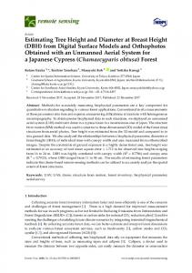
Figure 1. q-exponential function (6) properties when aq = a = 0.1 .

(8)

where

(1 − exp((1 − q)a1 x))

1 1−q

(9)

+

The Equation (8) recovers most one-species (logistic-like) models. The behaviour of the q-exponential function defined by Equation (6) for different q values and for a q = a = 0.1 can be found in Figure 1. As we can see from Figure 1, when q > 1 the q-exponential function grows faster than the ordinary exponential function, and when q < 1 the function grows slowly (if a q = a > 0

β1 − β 4

are parameters estimated from the data.

Volume models The wealth of allometric equations that relate stem volume to diameter at breast height and to tree height has been summarised for European tree species (Zianis et al., 2005). Four alternative models (described below) were used to predict stem volume: the three-parameter Schumacher and Hall (1933) model (Equation (14)), the two-parameter Honer (1965) model (Equation (15)), the six-parameter Meyer (1934) model (Equation (16)), and the sixparameter q-exponential model (Equation (17)).

V = β1Dβ2 Hβ3

(14)

Height models In this paper, four alternative models (described below) were used for the height–diameter relationship: the three-parameter Hill (1913) model (Equation (10)), the three-parameter Korf (Lundqvist, 1957) model (Equation (11)), the three-parameter Chapman-Richards model (Richards, 1959; Chapman, 1961) (Equation (12)), and the four-parameter q-exponential model (Equation (13)). These models were chosen because they have been found to perform better overall than many other height-diameter models.

D2

(10)

β2

(11)

(1 − β 3 )D β −1 3

(−β2D)) H=β1(1−exp

β3

β H = β 1 − 2 (1 − exp ((1 − β 4 )β 3 D )) β3

(12) 1 1− β 4 +

(13)

(15)

β1 + β 2 H

V = β1 + β 2 D + β3 D 2 + β 4 DH + β5 D 2 H + β 6 H

V = β1H

β D β2 H= 1 β β3 + D 2 H = β1 exp

V=

where

β2

β β 3 − 4 (1 − exp((1 − β 6 )β5 D)) β5

β1 − β6

1 1−β6

(16)

(17)

+

are parameters estimated from the data.

Taper models The main purpose in developing a stem profile model is to predict the diameter outside bark along the bole in terms of diameter outside bark at breast height and total height. The most commonly used stem profile models were developed by Max and Burkhart (1976) and Kozak (1988, 2004). In this study, three known taper models and one newly developed model were evaluated. Sharma and Parton’s (2009) variable-exponent single continuous function taper model was written as:

2372

Int. J. Phys. Sci.

H −h d = β1D H − 1 . 37

( ) prediction for total stem volume, V (D, H ) , in the following form:

equation of stem diameter, d = d D, H , h , allows us to revise the

β2 +β3z+β4z2

H 1 . 37

(18)

Where

h z= H d is the diameter outside bark at a given height h , D is the diameter outside bark at breast height, H is the total tree height from ground to tip, β1 − β 4 are parameters estimated from the

V (D , H ) =

H

π 40000

2

(d (D , H , h ))

⋅ dh

(22)

0

Statistical analysis and comparison of model performance

data.

In the general formulation of the nonlinear and linear fixed-effects models (Equations (10)-(21)) used in this study, the error terms ei

A few different formulations of taper models were proposed by Kozak (1988, 2004). In this study, one variable-exponent single continuous function taper model was utilised in the following form (Kozak, 2004):

(for height, volume and taper models) are assumed to be independent and identically distributed with means of zero and non constant variance. A power variance function was incorporated for the height, stem volume and taper models. Following Harvey (1976), we shall refer to it as the multiplicative heteroscedastic

d = β1 D β 2 H β 3 X

(

)

β 4 z 4 + β 5 exp − D H + β 6 X 0.1 + β 7 D −1 + β 8 H Q + β 9 X

(19) where

X =

(1 − h H ) (1 − p )

Q = 1− z p = 1.3

β1 − β9

1

1

3

3

1 3

H

d = β1Dβ2 (1−z) β1 − β5

β3z2+β4z+β5 (20)

are parameters estimated from the data.

A new segmented taper model was defined in the following form using a q-exponential function and parabola:

(

)

β 3 (z − 1 ) + β 4 z 2 − 1 , if z ≥ α 1 β2

β5 −

β6 (1 − exp β7

((1 −

β 8 )β 7 z ))

1 1− β 8 +

(21)

β1 − β8

ni × ni

matrix, Ri

(ρ ,σ ) , is

expressed as:

β 1 , β 2 , β 3 , β 5 > 0, β 4 < 0

where

γ is the variance function coefficient, D is the variance

covariate (diameter outside bark at breast height). The variance function coefficient γ was estimated by the modified two-step

the within-tree (i) variance-covariance

are parameters estimated from the data.

d = β1D

where

σ i2 = σ 2 D 2γ ,

procedure proposed by Harvey (1976). Equations (10)-(17) were fitted to the observed data using weighted least-squares regression (Non-linearFit procedure, LinearFit procedure for Equation (16)) in the symbolic computational language MAPLE. For taper Equations (18)-(21), fitting to improve estimation efficiency was accomplished using a generalised least squares technique (GLS) to account for correlations in the longitudinal data. In practice, certain assumptions must be imposed on the variancecovariance matrix so that a feasible GLS estimator can be computed. In order to achieve convergence, within-tree autocorrelation is not easy to justify. Here, a special structure for

The variable-exponent single continuous function taper model constructed by Lee et al. (2003) was defined as:

where

model. The power variance function was defined as

Ri (ρ ,σ ) = σ 2

1

ρ

ρ

1

0

0

0

.

1

The correlation structure is defined by the first-order autoregressive process AR(1), and it is assumed that ρ = ρ1 . All models were compared to the observed data. Numerical and graphical analyses of the residuals were used as criteria for comparing the models. The performance statistics of the height, stem volume and taper equations included four statistical indices: mean prediction bias (B), relative error in prediction (RE%), Akaike’s information criterion (AIC), and an adjusted coefficient of 2

determination ( R ):

B=

1 n

n

∧

yi − yi

i =1

are parameters estimated from the data.

The main advantage of using taper curves is that, if tree profiles can be described accurately, the volume for any merchantability segment can be computed using integration. Hence, the taper

0

ρ

n

RE% =

1 ⋅ n− p

∧

yi − yi

i =1

y

2

Rupšys and Petrauskas

2373

Table 2. Estimated parameters (standard errors in parentheses) of all models applied to the stem analysis data set. β6

β7

β8

β9

λ

-

-

-

-

-

-

-

-

-

-

-

-

-

-

-

-1.1642 (0.1845)

-

-

-

-

-

0.2595 (0.0079) 0.2592 (0.0079) 0.2599 (0.0079) 0.2590 (0.0079)

Eq.

β1

β2

β3

β4

(10)

43.8402 (3.2539) 62.0022 (7.4319) 32.1601 (0.9581) -206.4340 (102.722)

1.0482 (0.0596) 2.5435 (0.4279) 0.0396 (0.0039) 20.7527 (9.0234)

29.9976 (1.9284) 1.4933 (0.0538) 0.9879 (0.0560) -0.0041 (0.0021)

-

-9.6556 (.0.0424) 270.484 (197.47) 0.0681 0.0175) 0.0188 (0.0008)

1.8254 (.0.0113) 21206.4 (5356.6) .-0.0043 (.0.0022) 1.0016 (0.0125)

1.0068 (.0.0191) -

-

0.00005 -5 (6*10 ) 0.3235 (0.1473)

0.0008 -5 (8*10 ) 0.1342 (0.0120)

-0.3872 (0.0042) 0.8523 (0.0075) 1.3710 (0.0019) 1.5176 (0.0092)

0.8982 (0.0070) 0.9180 (0.0025) 0.9501 (0.0014) 0.9227 (0.0012)

0.0611 (0.0027) 0.1343 (0.0043) 3.0183 (0.0276) 1.2343 (0.0196)

-0.1886 (0.0026) 0.4189 (0.0040) -4.2443 (0.0351) -1.5620 (0.0119)

(11) (12) (13)

(14) (15) (16) (17)

(18) (19) (20) (21)

AIC = n ln(RSS) + 2 p , RSS =

n

∧

β5

Height models -

Volume models -

-

-

-

-

-

-

-

-

-

0.00002 -6 (2*10 ) -0.0723 (0.0336)

-0.0087 (0.0011) 0.7203 (0.0733)

-

-

-

-

-

-

Taper models 0.5495 (0.0037) -0.1785 0.4089 (0.0148) (0.0035) 2.1725 (0.0115) 0.5620 -7.2536 (0.0276) (0.4475)

2

2

R = 1−

n − 1 i =1 n n− p

∧ yi − yi

0.9853 (0.0079)

-

-

-

0.2142 (0.0939) -

-0.0002 (0.0004) -

0.0296 (0.0062) -

-0.7334 (0.0247)

13.3801 (0.7618)

-

0.1519 (0.0023) 0.1148 (0.0022) 0.1526 (0.0022) 0.1190 (0.0023)

achieves the minimum AIC in the class of the competing models.

yi − yi

i =1 n

0.8582 (0.0079) 1.4036 (0.0079) 0.6876 (0.0079)

2

(yi − y )2

i =1

where n is the total number of observations used to fit the height, stem volume and taper models, p is the number of model ∧

parameters, yi , yi , and y are the measured, estimated and average values of the dependent variable (height, stem volume, diameter outside bark), respectively. The AIC can generally be used for the identification of an optimum model in a class of competing models (Akaike, 1974). The first term on the right hand side of AIC equation is a measure of the lack-of-fit of the chosen model, while the second term measures the increased unreliability of the chosen model due to the increased number of model parameters. The best approximating model is the one which

RESULTS AND DISCUSSION The parameters of all models used to analyse the data set summarised in Table 1 are presented in Table 2. All parameters are highly significant ( α < 0.05 ), with the exceptions of Honer’s volume model (15) (parameter β1 )

and Kozak’s model (19) (parameter β 8 ). For the qexponential segmented taper model defined by Equation (21), a joint point was calculated at 0.52, as the fit statistics obtained the best values. The results of goodness of fit statistics for all models applied to the stem analysis data set are summarised in Table 3. In general, height models account for at least 75% of the variation in height, volume models account for at least 98% of the variation in volume, and the taper models account for at least 98% of the variation in diameter outside bark (Table 3). Fit characteristics (RE%, AIC, R 2 ) of

2374

Int. J. Phys. Sci.

Table 3. Estimation goodness of fit statistics for all models applied to the stem analysis data set.

Equation

B

RE%

AIC

R

2

Height models (10) (11) (12) (13)

-0.0023 0.0001 -0.0002 0.0252

12.91 12.89 12.94 12.88

18338 18332 18346 18329

0.750 0.751 0.749 0.751

(14) (15) (16) (17) (18) and (22) (19) and (22) (20) and (22) (21) and (22)

-0.0001 -0.0028 -6 9.3*10 -0.0001 -0.0032 0.0073 0.0003 0.0065

Volume models 11.51 12.76 11.37 11.24 13.03 11.59 12.22 11.58

4346 4740 4301 4257 4822 4377 4578 4373

0.984 0.981 0.985 0.985 0.980 0.984 0.983 0.985

(18) (19) (20) (21)

-0.0932 0.0280 0.0563 0.0180

Taper models 10.37 7.89 8.89 7.79

279342 265881 271736 265221

0.973 0.984 0.980 0.985

the q-exponential height model (13) gave better results than the other models used here. In terms of all fitness statistics used, the q-exponential model (17) appears to best predict stem volume. In terms of all fitness statistics used, the q-exponential segmented taper model (21) appears to best predict diameter outside bark. The proposed taper Equations (18)-(21) can be directly integrated (Equation (22)) between 0 and H to obtain stem volume. By using taper Equations (18)-(21), the predictive ability of stem volume is similar to a simple regression models (14)-(17) (Table 3). The final step in evaluating the various models involved visual examinations of studentized residuals against the predicted values (height and volume models) and the relative height (taper models). Figures 2 and 3 show the studentized residuals plotted against predictions of height and volume, respectively. Figure 4 shows the studentized residuals plotted against relative heights. Graphical diagnostics of studentized residuals for the height predictions indicated that the residuals of the q-exponential and Korf models displayed more homogeneous variance than the other height models (Figure 2). Studentized residuals plots (Figure 3) for the stem volume predictions demonstrated that the q-exponential and Meyer models are superior to other models in predicting the stem volume. The plots of the studentized residuals for the diameter predictions indicated that the residuals of the q-exponential and Kozak models displayed more homogeneous variance than the

other models (Figure 4). These results are very similar to the conclusions drawn based on fitness statistics. However, for stem volume predictions, the residuals increased steadily with predicted stem volume. The trend becomes less obvious when the predicted 3 volume is less than 1.5 m . The height-diameter and volume-diameter-height relationships of a tree species are highly site-dependent and non constant over time. Incorporating datasets observed from different plots into a single comprehensive analysis introduces some inhomogeneity and affects the resulting predictions. To account for stand-level variation, Misir (2010), Sharma and Zhang (2004) and Cienciala et al. (2006) generalized these relationships using stand characteristics, Comparing several models, they concluded that the generalized models were very similar in terms of statistical indexes (relative error in prediction and adjusted coefficient of determination). The ChapmanRichards growth model has been widely used in the modelling a number of tree species. Peng et al. (2001) and Berrill and Hay (2006) examined the performance of the Chapman-Richards model to predict tree height for nine boreal forest tree species in Canada and four tree species of eucalypt stands in New Zealand, respectively. They recommended the Chapman-Richards curve for these tree species on the basis of its satisfactory prediction performance. Zianis et al. (2005) compiled 230 stem volume equations and they covered 55 species altogether. In the majority of the compiled stem volume

Rupšys and Petrauskas

Figure 2. Studentized residuals for the height models.

Figure 3. Studentized residuals for the stem volume models.

2375

2376

Int. J. Phys. Sci.

Figure 4. Studentized residuals for the stem profile models.

models the independent variables were diameter at breast height and/or height. Taper models presented by Kozak (1988, 2004) are examples of simple taper functions. Kozak and q-exponential taper models were very competitive in terms of estimated adjusted coefficient of determination and relative error in prediction. To further improve predictions by q-exponential models, a first step could be to detect and model a variance function and add new predictors such as stand density and crown-length ratio. A second step could be to apply mixed-effects models (Sharma and Parton, 2009; Li and Weiskittel, 2010) and stochastic differential equations methodology (Rupšys and Petrauskas, 2010a, b; Rupšys et al., 2011). Figure 5 plots taper profiles obtained using four different taper equations (Equations (18)-(21)) for three randomly selected pine trees with diameters outside bark at breast height of 19.6, 38.2, and 45.2 cm and with total tree heights of 19.1, 22.4, and 31.9, respectively. All tapers correlated well with the stem data. The shapes of the taper curves (Figure 5) are sufficiently similar that measures such as residual sums of squares are unlikely to distinguish the four taper equations, given the data set used here. Graphical examination leads to the conclusion

that the q-exponential segmented taper model (21) describes stem profile quite well and is superior to the other taper models. Conclusions The q-exponential function was modified to model tree height, volume and stem profile. We compared performance among various previously constructed models of tree height, volume and stem profile in the context of Scots pine (P. Sylvestris) data. Fitness characteristics of the q-exponential models were better than those of other models. The q-exponential function presented in this study represents a general framework that can be applied to other model forms and response variables of trees or stands. ACKNOWLEDGEMENT The authors would like to thank the referees for their careful reading of the manuscript. This work was supported in part by the Lithuanian Association of Impartial Timber Scalers.

Rupšys and Petrauskas

2377

Figure 5. Tree profiles for three randomly selected pine trees generated using Sharma-Parton (18), Kozak (19), Lee et al. (20) and q-exponential segmented (21) taper models.

REFERENCES Abe S, Okamoto Y (2001). Nonextensive Statistical Mechanics and Its Applications. Springer, Berlin. Akaike H (1974). A new look at the statistical model identification. IEEE Trans. Automatic Control, 19: 716-723. Berrill JP, Hay AE (2006). Indicative growth and yield models for stringybark eucalypt plantations in northern New Zealand. New Zealand J. For. 51(1): 19-22. Chapman DG (1961). Statistical problems in dynamics of exploited fisheries populations. In: Neyman, J. (ed.) Proceedings of 4th Berkeley Symposium on Mathematical Statistics and Probability, Berkeley: CA, 4: 153-168. Cienciala E, erny M, Tatarinov E, Apltauer J (2006). Biomass functions applicable to Scots pine. Eur. J. Forest Res. 20: 483-495. Ferri GL, Reynoso Savio MF, Plastino A (2010). Tsallis' q-triplet and the ozone layer. Physica A, 389: 1829-1833. Gompertz B (1825). On the nature of the function expressive of the law of human mortality, and on a new mode of determining the value of

life contingencies. Phil. Trans. R. Soc., 115: 513-585. Gontis V, Ruseckas J, Kononovi ius A (2010). A long-range memory stochastic model of the return in financial markets. Physica A, 389: 100-106. Harvey AC (1976). Estimating regression models with multiplicative heteroscedasticity. Econometrica, 44: 461-465. Hill VA (1913). The combinations of hemoglobin with oxygen and with carbon monoxide. Biochem. J., 7: 471-480. Honer TG (1965). A new total cubic foot volume function. Forestry Chronicle 41:476-493. Kozak A (1988). A variable-exponent taper equation. Can. J. For. Res., 18: 1363-1368. Kozak A (2004). My last words on taper equations. Forestry Chronicle, 80: 507-514. Lee WK, Seo JH, Son YM, Lee KH, Gadov K (2003). Modeling stem profiles for Pinus densiflora in Korea. For. Ecol. Manage., 172: 69-77. Li R, Weiskittel AR (2010). Comparison of model forms for estimating stem taper and volumes in the primary conifer species of the North American Acadian Region. Ann. For. Sci., 67: 302.

2378

Int. J. Phys. Sci.

Lithuanian Statistical Yearbook of Forestry (2009). Ministry of Environment, State Forestry Survey Service, p. 152. Lundqvist B (1957). On the height growth in cultivated stands of pine and spruce in Northern Sweden. Medd. Fran Statens Skogforsk. Band, 47: 1-64. Marshall PL, Lencar C, Hassani B (2000). Review of PSP Systems Employed Outside of British Columbia. University of British Columbia, Vancouver, p. 58. Max TA, Burkhart HE (1976). Segmented polynomial regression applied to taper equations. For. Sci., 22: 283-288. Mensah FE, Grant JR, Thorpe AN (2010). The evolution of the molecules of deoxy-hemoglobin S in sickle cell anaemia: A mathematical prospective. Int. J. Phys. Sci., 4: 576-583. Meyer HA (1934). Die rechnerischen Grundlagen der Kontrollmethode. Beiheft zu den Zeitschriften der Forstvereins, 13: 122. Misir N (2010). Generalized height-diameter models for Populus tremula L. stands. Afr. J. Biotechnol, 9: 4348-4355. Peng C, Zhang L, Liu J (2001). Developing and validating nonlinear height-diameter models for major tree species of Ontario’s boreal forests. North. J. Appl. For., 18: 87-94. Richards FJ (1959). A flexible growth function for empirical use. J. Exp. Bot., 10: 290-300. Rupšys P, Bartkevi ius E, Petrauskas E (2011). A univariate stochastic Gompertz model for tree diameter modelling, Trends in Appl. Sci. Res., 6: 134-153. Rupšys P, Petrauskas E (2010). Quantyfying tree diameter distributions with one-dimensional diffusion processes. J. Biological Syst., 18: 205-221. Rupšys P, Petrauskas E (2010b). The bivariate Gompertz diffusion model for tree diameter and height distribution. For. Sci., 56: 271280. Salazar S, Sanchez LE, Galindo P, Santa-Regina I (2008). Aboveground tree biomass equations and nutrient pools for a paraclimax chestnut stand and for a climax oak stand in the Sierra de Francia Mountains, Salamanca, Spain. Sci. Res. Essays, 5: 1294-1301.

Schumacher FX, Hall FDS (1933). Logarithmic expression of timber tree volume. J. Agric. Res., 47: 719-734. Sharma M, Parton J (2009). Modeling stand density effects on taper for jack pine and black spruce plantations using dimensional analysis. For. Sci., 55: 268-282. Sharma M, Zhang SY (2004). Height-diameter models using stand characteristics for Pinus banksiana and Picea mariana. Scand. J. For. Res., 19: 442-451. Sloboda BV, Gaffrey D, Matsumura N (1993). Regionale und lokale Systeme von Höhenkurven für gleichalrigeWaldbestände. Allgemeine Forst- und JagdZeitung, 164: 225–228. Souto Martinez AS, Silva González RS, Lauri Espíndola AL (2009). Generalized exponential function and discrete growth models. Physica A, 388: 2922-2930. Strzalka D, Grabowski F (2008). Towards possible q-generalizations of the Maltus and Verhulst growth models. Physica A, 387: 2511-2518. Tsallis C (1988). Possible generalization of Boltzmann-Gibbs statistics. J. Statist. Phys., 52: 479-487. Tsallis C (2004). What should a statistical mechanics satisfy to reflect nature? Physica D: Nonlinear Phenomena, 193: 3-34. Upadhyayaa A, Rieub JP, Glaziera JA, Sawadac Y (2001). Anomalous diffusion and non-Gaussian velocity distribution of Hydra cells in cellular aggregates. Physica A, 293: 549–558. Verhuulst PF (1838). Notice sur la loi que la population suit dans son accroissement. Correspondence Mathematiue et Physique publie par A Quetelet, 10: 113-121. von Bertalanffy L (1938). A quantitative theory of organic growth. Hum. Biol. 10: 181-213. Zianis D, Muukkonen P, Mäkipää R, Mencuccini M (2005). Biomass and stem volume equations for tree species in Europe. Silva Fennica Monographs, 4: 1-63.