Development of robust calibration models in near infra-red spectrometric applications. H. Swierengaa, F. Wülfertb, O.E. de Noordc, A.P. de Weijerd, A.K. Smildeb ...
Analytica Chimica Acta 411 (2000) 121–135
Development of robust calibration models in near infra-red spectrometric applications H. Swierenga a , F. Wülfert b , O.E. de Noord c , A.P. de Weijer d , A.K. Smilde b , L.M.C. Buydens a,∗ a
c
Laboratory of Analytical Chemistry, Faculty of Science, Catholic University of Nijmegen, Toernooiveld 1, 6525 ED Nijmegen, The Netherlands b Department of Chemical Engineering, Process Analysis & Chemometrics, University of Amsterdam, Nieuwe Achtergracht 166, 1018 WV Amsterdam, The Netherlands Shell International Chemicals B.V., Shell Research and Technology Centre, P.O. Box 38000, 1030 BN Amsterdam, The Netherlands d Akzo Nobel Central Research, P.O. Box 9300, 6800 SB Arnhem, The Netherlands Received 3 November 1999; accepted 13 January 2000
Abstract When spectral variation caused by factors different from the parameter to be predicted (e.g. external variations in temperature) is present in calibration data, a common approach is to include this variation in the calibration model. For this purpose, the calibration sample spectra measured under standard conditions and the spectra of a smaller set measured under changed conditions are combined into one dataset and a global calibration model is calculated. However, if highly non-linear effects are present in the data, it may be impossible to capture this external variation in the model. Recently, a new technique, which is based on selection of robust variables, was proposed for constructing robust calibration models. In this technique, a calibration model is developed which uses a subset of spectral values that are insensitive to external variations. This new technique is compared with global calibration models for constructing robust models in spectrometric applications. Both techniques are applied to two different near infra-red (NIR) spectroscopic applications. The first is the determination of the ethanol, water, and iso-propanol concentrations in a ternary mixture of these components; the second is the determination of the density of heavy oil products. In both applications, the calibration set spectra have been measured at a standard sample temperature and a subset has been measured at sample temperatures deviating from the standard temperature. It has been found that models based on robust variable selection are similar or sometimes better than global calibration models with respect to their predictive ability at different sample temperatures. © 2000 Elsevier Science B.V. All rights reserved. Keywords: Robust calibration; Near infra-red spectrometry
1. Introduction Multivariate calibration models are often associated with vibrational spectroscopic techniques in order to predict physical or chemical sample properties from ∗ Corresponding author. Tel.: +31-20-525 5062; fax: +31-20-525 5604.
the spectra. To construct a multivariate calibration model, the spectra and corresponding properties of many samples need to be measured in order to capture the variation in the sample properties to be predicted. Once the model has been developed, it is supposed to be valid for a long period of time. This implies that, after this period, the model’s prediction error is not significantly different from the prediction error
0003-2670/00/$ – see front matter © 2000 Elsevier Science B.V. All rights reserved. PII: S 0 0 0 3 - 2 6 7 0 ( 0 0 ) 0 0 7 1 8 - 2
122
H. Swierenga et al. / Analytica Chimica Acta 411 (2000) 121–135
obtained during calibration. However, there may be various reasons why the model makes erroneous predictions: replacement of the instrument or part of it, ambient changes such as temperature, and changes in physical sample conditions [1]. If the calibration model loses its validity, a new calibration model needs to be constructed. Therefore, a set of calibration samples, representative of the original calibration samples, should be remeasured under the changed conditions. If the original calibration samples are not stable, this calls for collecting or preparing new samples, measuring the reference values and measuring the corresponding spectra, which may involve a large amount of work. Recently, more efficient methods, known as multivariate calibration standardization methods, became available to establish a new calibration model [1]. Multivariate calibration standardization methods can be divided into two categories: (1) improvement of robustness of the calibration model; and (2) adaptation of the calibration model [2]. The first category aims at improving the selectivity of the calibration model by data preprocessing (e.g. variable selection), the incorporation of measurement conditions into the calibration model (global calibration models) and/or the application of robust multivariate calibration techniques such as variable selection partial least squares (IVS-PLS) [3]. The second category includes techniques that transform the measured spectra, the model’s regression parameters or the predictions by the calibration model (e.g. bias/slope correction, direct standardization and piecewise direct standardization). One of the disadvantages of this category is that the same sample subset needs to be measured in both the old and the new situation, which is not possible when unstable samples are involved. Another disadvantage of techniques of Category 2 is that they are only applicable to discrete situations such as instrumental changes. Frequently, however, external conditions (e.g. sample temperature) which influence the model’s predictions change continuously, and consequently, techniques of Category 2 cannot be applied. In the applications studied in this paper, the sample temperature is a continuously changing condition, and we therefore focused on two techniques of the first category: (A) global calibration models; [4] and (B) robust variable selection models [5]. Although often not recognized, global calibration models are used frequently. The construction of a
global calibration model involves measurement of calibration samples under normal conditions, measurement of these samples or a sample subset under changed conditions and the combination of the data to one dataset. Besides spectral variation caused by the variation in the reference parameter, this dataset includes external spectral variation introduced by the new situation. Subsequently, a new calibration model is calculated on the basis of the joint dataset. Thus, global calibration models try to model the external spectral variation and implicitly include the external variation into the calibration model. Recently, a new technique based on variable selection was presented in order to enhance the robustness of a calibration model [5]. Instead of using the whole spectral range for modeling, this technique uses a subset of spectral values which is not sensitive to the changing conditions and rejects those spectral regions that are sensitive to these changing conditions. There are various reasons why the predictive ability and the robustness of a calibration model are enhanced by variable selection: (1) some spectral regions related to the parameter of interest may contain large variation caused by external influences such as temperature variations or interferents; (2) there may be spectral regions whose intensities (absorbances) are not linearly related to the parameter to be predicted; and (3) there may be spectral regions which exhibit an indirect correlation with the parameter of interest (apparent causalities). This makes variable selection especially suitable for situations in which the spectral variation caused by external changes are localized in the spectra. Thus, instead of modeling the external variation, robust variable selection excludes external spectral variation before modeling. In this paper, global calibration models are compared with the new technique for enhancement of model robustness, namely calibration models based on robust variable selection. In order to select the robust variables, simulated annealing (SA) was used. Both techniques were applied to two near infra-red (NIR) spectroscopic applications. The first is the determination of the ethanol, water, and iso-propanol concentrations in a ternary mixture of these components; the second is the determination of the density of heavy oil products. In both applications, the model’s predictions should be insensitive to sample temperature variations within a predefined temperature range. In this paper,
H. Swierenga et al. / Analytica Chimica Acta 411 (2000) 121–135
only PLS regression models are considered, but the above-mentioned techniques can be applied to other multivariate calibration techniques as well. 2. Theory 2.1. Global calibration models Global models try to include implicitly the variation due to external effects in the model, in much the same way as unknown chemical interferents can be included in an inverse calibration model. As long as the interfering variation is present in the calibration set, an inverse calibration model can, in the ideal case of additivity and linearity, easily correct for the variation due to the unknown interferents. It is assumed in global calibration models that the new sources of spectral variation can be modeled by including a limited number of additional PLS factors [4]. Owing to increase in the calibration model’s dimensionality, it becomes necessary to measure a large number of samples under changed conditions in order to make a good estimation of the additional parameters [6]. When highly non-linear effects are present in the spectra, many additional PLS factors will be necessary to model the spectral differences, and sometimes, it is not possible to model these spectral differences. Therefore, other strategies need to be used to make modeling of non-linear data possible [7]. 2.2. Robust variable selection models Whereas global models try to capture the external variation into the model, robust variable selection attempts to exclude the external variation before modeling. Basically, it selects those spectral regions that are important for the parameter to be predicted and those that can correct for the spectral differences caused by external conditions, at the same time rejecting those regions that are sensitive to the spectral differences caused by the external variations. It is assumed that a calibration on the robust wavelengths will be free of influences of external factors and may be more parsimonious, as it only needs to model the spectral variation caused by the parameter of interest. However, it is difficult to compare variable selection with other calibration models with respect to parsimony because
123
it is difficult to assess the degrees of freedom lost in the selection of the robust variables (many models are calculated during optimization) [8]. While global calibration models are straightforward and the model calculations can be performed in a short time by commercially available software packages, the robust variable selection by SA requires more sophisticated software and faster computers. Furthermore, some additional parameters need to be optimized for the SA algorithm (number of PLS factors, the number of variables selected, representation of problem, length of Markov chain, initial temperature, or control parameter). Therefore, special expertise about the SA techniques is necessary. Since the number of selected variables will be seriously reduced and a lot of models are calculated during optimization, chance of overfitting exists; the selected variable subset should not include irrelevant noise-containing variables and overfitting should be prevented. Recently, Jouan-Rimbaud et al. developed a method to evaluate the performance of variable selection by genetic algorithms (GAs) with respect to overfitting [9]. For this purpose, they added random variables to the original spectral data matrix and performed a GA run using this extended dataset. The number of random selected variables is a measure for the selection of randomly correlated variables from the original spectral data. Leardi et al. proposed a stop criterion for a variable subset search by a GA in order to prevent overfitting [10]. This stop-criterion is based on a random permutation test of the original Y variables. All problems associated with robust variable selection result from the use of SA and not from the principle of using a spectral subset for PLS modeling instead of using the whole spectral range. If knowledge would be available about the relation between external variables and the spectral intensities, these problems would disappear. Usually, however, no physical model is available for estimating the influence of external variations on the spectral variables. As a result, variable selection techniques need to be used to make the spectral subset selection. 2.3. Simulated annealing Since no prior knowledge is available, the selection of the robust variables out of the whole spectral range
124
H. Swierenga et al. / Analytica Chimica Acta 411 (2000) 121–135
is a large optimization problem which can be solved by optimization techniques such as SA or GAs. In this paper, SA is used for variable selection. SA is a probabilistic global optimization technique, based on the physical annealing process of solids. In contrast to deterministic optimization techniques (e.g. simplex optimization), probabilistic optimization techniques allow acceptance of an inferior solution during optimization. Consequently, probabilistic optimization techniques have the ability to escape from a local optimum and to find the global optimal solution. More detailed description about SA can be found in the literature [5,11]. An SA solution is represented as a numerical string containing k values (integers) representing the variables to be selected from the whole spectral range of N variables. These k variables are selected from the calibration set spectra, and in combination with reference values of the corresponding samples, a PLS model with a predefined number of factors is calculated. Subsequently, the same k variables are selected from the standardization set spectra (spectra measured under changed circumstances) and the reference parameters are predicted using the calibration set and the standardization set variable subset spectra. On the basis of these prediction results, an error value is calculated. This error value comprises the predictive ability of the model at the standard temperature and the predictive ability of the model when it is used at different temperatures. The goal of SA is to minimize the error value; which implies that the prediction error of the model is minimized at all temperatures. In order to find the proper k value, various SA runs are performed using different values for k. 2.4. Comparison of predictive accuracy of models Usually, two models are compared with respect to their predictive ability on a representative independent data set (i.e. dataset not used for model calculation). Frequently, the predictive ability of a model is expressed in the mean squared error of prediction (MSEP). During the development of a calibration model, a minimal MSEP value is aimed at. Recently, Swierenga et al. proposed a strategy which uses the prediction error, and simultaneously, the sensitivity to external variations for selecting a multivariate calibration model [12]. Van der Voet proposed a
randomization t-test to compare the predictive accuracy of two models using the distribution of prediction errors [13]. In this paper, this randomization t-test is applied in order to compare the predictive ability of global models and robust variable selection models.
3. Experimental 3.1. Dataset A: ternary mixture of ethanol water and iso-propanol The mixtures (19 samples) were prepared from p.a. quality alcohols and sub-boiled water according to a mixture design (Fig. 1) [4]. Short-wavelength NIR measurements (580–1091 nm, 1 nm resolution, 20 s integration time) were performed on a Hewlett–Packard HP 8453 spectrophotometer with a thermostatable cell holder and a cell stirring module. Closed quartz cells with 1 cm path length were used with an external Pt-100 sensor immersed in the sample linked to a circulator bath for temperature control and measurement. Instrumental baseline drift and offset of the spectra was corrected with straight line fits using the wavelength range 749–849 nm. The data analysis was performed in the region 850–1049 nm. The spectra of these 19 ternary mixtures of ethanol, water and iso-propanol were measured at 50◦ C. The dataset was split into a calibration set (Fig. 1A) containing samples 1, 2, 3, 4, 7, 8, 10, 12, 13, 16, 17, 18, 19 and a test set (Fig. 1C) containing samples 5, 6, 9, 11, 14, 15. The calibration set will be denoted by 50 and the test set as X 50 . A subset of the calibraXcal test tion set (Fig. 1B) containing samples 1, 3, 8, 10, 12, as test 17, 19 was measured at 30, 40, 60, and 70◦ C 30 , X 40 , X 60 , X 70 , and will be denoted by Xstand stand stand stand respectively. The test set samples were measured at the same temperatures and will be denoted by 30 , X 40 , X 60 , X 70 , respectively. These datasets Xtest test test test were used to calculate and validate the global calibration model and the calculation of a model containing robust wavelengths. 3.1.1. Local calibration model Local models were built to evaluate the influence of temperature on the model’s predictions if temperature effects are not taken into account at all. Therefore, a
H. Swierenga et al. / Analytica Chimica Acta 411 (2000) 121–135
125
PLS1 calibration model was calculated based on the 50 . The number of PLS factors is four which spectra Xcal was determined by leave-one-out cross-validation. The 30 , X 40 , X 50 , X 60 , and X 70 were used datasets Xtest test test test test as independent test sets. 3.1.2. Global calibration model 30 , X 40 , X 50 , X 60 , and X 70 Datasets Xstand stand cal stand stand were used to calculate global calibration (PLS1) mod30 , X 40 , X 50 , X 60 , and X 70 els and datasets Xtest test test test test were used as independent test sets. The number of PLS factors for the model was determined by leave-one-sample-out cross-validation and the optimal model complexity is seven factors for all three components in the ternary mixtures. 3.1.3. Robust variable selection Out of the whole set of possible variables (200 variables), a subset of k variables was proposed as a possible solution by the SA algorithm. This subset of 50 , and a PLS variables was selected from the dataset Xcal model was calculated using four PLS factors (number of factors for local models). Subsequently, this model was used to make predictions of the contents using the 30 , X 40 , X 60 , and X 70 . spectra from sets Xstand stand stand stand On the basis of the prediction results, an error value was calculated representing the predictive ability of the model at various temperatures (30, 40, 50, 60 and 70◦ C). During an SA run, this error value was minimized. At the end of the SA search, the calculated model was tested using the independent datasets 30 , X 40 , X 50 , X 60 , and X 70 . Ten random iniXtest test test test test tialized SA runs were performed at a certain k value. 3.2. Dataset B: density of heavy oil products
Fig. 1. Construction of datasets used for multivariate calibration. (A) Calibration set measured at one temperature; (B) standardization set (subset of calibration set) measured at 30, 40, 60, and 70◦ C; (C) test set measured at 30, 40, 50, 60, and 70◦ C.
NIR spectra (6206–3971 cm−1 , 1.9 cm−1 data point and 3.8 cm−1 spectral resolution) of the heavy oil products were measured on a Bomem MB 160 FTNIR spectrometer in a temperature controlled flow cell. The density measurements were performed following the ASTM D4052 method. Baseline offset correction of the spectra was applied by subtracting the average absorbance in the range 4810–4800 cm−1 . The last 400 variables (4740–3971 cm−1 ) were used for the data analysis.
126
H. Swierenga et al. / Analytica Chimica Acta 411 (2000) 121–135
The spectra of 42 heavy oil samples were measured at 100◦ C. This calibration set of 42 samples will be 100 . Subsequently, 15 samples were sedenoted by Xcal lected from the calibration set using the Kennard Stone algorithm [14,15] and this subset was measured at 95 and 105◦ C. These standardization sets will be denoted 95 105 , respectively. Furthermore, a test by Xstand and Xstand set containing 35 samples was measured at 95, 100, and 105◦ C and the test set spectra will be denoted as 95 100 , and X 105 , respectively. , Xtest Xtest test 3.2.1. Local model 100 was used to calculate the local model Dataset Xcal for the prediction of density. The model complexity was determined by leave-one-out cross-validation and 95 100 , and X 105 , Xtest was set to five factors. Datasets Xtest test were used as independent test sets. 3.2.2. Global calibration model 95 100 , and X 105 , Xcal Datasets Xstand stand were used to calculate a global calibration model and datasets 95 100 , and X 105 as independent test sets. The , Xtest Xtest test number of PLS factors for the model was determined by leave-one-sample-out cross-validation and the optimal model complexity is six factors. 3.2.3. Robust variable selection Out of the whole set of possible variables (400 variables), a subset of k variables was proposed as a possible solution by the SA algorithm. This subset 100 , and of variables was selected from the dataset Xcal a PLS model was calculated for these spectral variables and the corresponding density using five PLS factors. Subsequently, this model was used to make predictions about the density using the spectra of sets 95 105 . On the basis of the prediction re, and Xstand Xstand sults, an error value is calculated which represents the predictive ability of the model at various temperatures (95, 100, and 105◦ C). During an SA run, this error value was minimized. At the end of the SA search, the calculated model was tested using the indepen95 100 , and X 105 . Ten random ini, Xtest dent datasets Xtest test tialized SA runs were performed at a certain k value. 3.3. Model validation The test sets were used to validate the constructed 30 , X 40 , X 50 , X 60 , calibration models (dataset A: Xtest test test test
70 and dataset B: X 95 , X 100 , and X 105 ). These Xtest test test test datasets were used to predict the component concentrations in the ternary mixtures (dataset A) and the density in the oil samples (dataset B). The difference between the predicted and the reference values is expressed in the prediction error:
RMSEP =
N X (yˆn − yn )2 n=1
!1/2
N
where N is the number of samples in the test set; yˆn , and yn are the predictions and the reference values of the samples of the test set, respectively. 3.4. Software and algorithms For local and global models, MatlabTM [16] and the PLS Toolbox [17] for MatlabTM were used. For robust variable selection, an SA toolbox has been written in ANSI C. Additionally, some PLS routines from the PLS Toolbox for MatlabTM were integrated, using the MATCOM compiler (version 2). The programs were compiled for the DOS/Windows operating system using DJGPP, version 2.01. The configuration of SA for the different datasets is shown in Table 1. A detailed description of the configuration can be found in a previous paper [5]. 3.5. Randomization t-test The randomization t-test was performed in order to compare the test set prediction results of global models and models based on robust variable selection. To this end, for example the ternary mixtures, the component concentrations were predicted from spectra measured at various temperatures by the two models to be compared (global and robust variable selection model). Subsequently, two vectors were constructed from these predictions: one containing the global model predictions for one component at various temperatures and one containing the variable selection model predictions for the same component at various temperatures (vector containing number of temperatures times N elements, where N is the number of samples in the test set). These vectors, along with the known reference values, were used for the randomization t-test.
H. Swierenga et al. / Analytica Chimica Acta 411 (2000) 121–135
127
Table 1 Parameters for the different SA runs used in this paper SA parameter [5]
Number of spectral variables to select from (N) Disturbance generation Initial control parameter (c1 ) Cooling schedule Length of Markov chain Exit Markov chain
Exit SA Acceptance criterion
Application Component concentrations in ternary mixture
Density of heavy oil products
200
400
N (0, 5) 0.05 geometric with α=0.90 1000 minimum number of accepted transitions (250) or maximum number of transitions tested (1000) minimum control parameter c=1×10⁻⁶ or minimum acceptance ratio χ =0 Metropolis
N (0, 5) 0.01 geometric with α=0.85 1000 minimum number of accepted transitions (250) or maximum number of transitions tested (1000) minimum control parameter c=1×10⁻⁶ or minimum acceptance ratio χ =0 Metropolis
4. Results and discussion 4.1. Dataset A: ternary mixture of ethanol, water and iso-propanol 4.1.1. Temperature influence on vibrational spectra An NIR spectrum consists of overtones and combination bands (resulting from the interaction between two or more different vibrations of neighboring bonds). These absorption bands provide information about features such as chemical nature (e.g. bond types and functional groups) and molecular conformation (e.g. gauche- and trans-conformations). It provides information about the individual molecular bonds and information about the interaction between different types of molecules (intermolecular bonds). Since the molecular vibrations are influenced by these intermolecular interactions, absorption bands in mixtures change in relation to pure analytes. Usually, intermolecular interaction such as hydrogen bondings is very weak and can be broken by increasing the temperature. Consequently, the vibrational spectrum will change due to these temperature changes. In Fig. 2, the temperature effect on pure water spectrum is shown; an increase in the temperature results in an intensity increase, peak shift towards lower wavelengths, and band narrowing. As mentioned in [4], an increase in temperature results in a decrease in the number of hydroxyl groups involved in a hydrogen bonding, and consequently, the absorption band of ‘free’ hydroxyl increases. Also, the second overtone
absorption band of the hydroxyl group in ethanol and iso-propanol (∼970 nm) increases as the sample temperature increases. On the other hand, in both ethanol and iso-propanol spectrum, the third overtone C–H stretch (∼910 nm) of the CH3 group and the C–H stretch (third overtone at ∼920–930 nm) of the CH2 group in ethanol change slightly owing to tempera-
Fig. 2. Selected variables for the determination of ethanol, water, and iso-propanol content in ternary mixtures. Lower dots (pro.): selected variables (10) for determination of iso-propanol (10 SA runs); centre dots (eth.): selected variables (30) for determination of ethanol (10 SA runs); upper dots (wat.): selected variables (30) for determination of water (10 SA runs). Additionally, the NIR spectra of pure ethanol (—), water (– · –) and iso-propanol (– –) measured at 30, 40, 50, 60, and 70◦ C are plotted. A baseline of 0.075 absorbance (AU) was added to the ethanol spectra for visualization purposes.
128
H. Swierenga et al. / Analytica Chimica Acta 411 (2000) 121–135
Table 2 Prediction results for determination of ethanol content Model type
Local Local (50◦ C) Global Variable selectiona a
No. of variables
200 200 200 30
No. of PLS factors
4 4 7 4
RMSEP
RMSEP
RMSEP
RMSEP
RMSEP
30◦ C
40◦ C
50◦ C
60◦ C
70◦ C
0.018 0.063 0.014 0.007
0.011 0.028 0.012 0.011
0.017 0.017 0.037 0.023
0.010 0.043 0.016 0.015
0.011 0.079 0.014 0.009
Mean RMSEP
0.014 0.051 0.021 0.014
From 10 SA runs, the best model (smallest overall prediction error in standardization sets) is selected.
ture changes. Some increase in the C–H combination band of the CH3 group (∼1020 nm) in ethanol and iso-propanol is observed in the spectra when the temperature is increased. 4.1.2. Determination of ethanol content The test set prediction results of various PLS models for determination of the ethanol content are shown in Table 2. In the first row of Table 2, the test set prediction errors of the individual local models at each temperature are shown. These values are taken from [3]. Similar test set prediction results are observed in the models. Subsequently, the local model based on spectra measured at 50◦ C is used to make predictions from spectra measured at temperatures deviating from 50◦ C (second row, Table 2). The prediction error increases if the predictions are performed with samples measured at temperatures deviating from 50◦ C. Thus, the sample temperature influences the NIR spectra, and consequently, the model’s predictions. In order to make the model insensitive to temperature variations, a global model and robust variable selection models are constructed. For both the global model and the variable selection model, the prediction errors of the test set samples measured at different temperatures are shown (third and fourth rows,
Table 2). Since 10 SA runs were performed, 10 robust variable selection models were obtained. From these models, the model that possesses the smallest overall prediction error in the standardization sets is selected. The test set prediction errors (RMSEP values) obtained using the global model at different temperatures are compared with the predictions obtained using the variable selection model at those temperatures. The overall prediction error obtained using the variable selection model (overall RMSEP=0.014) is found to be significantly smaller than the overall prediction error obtained using the global model (overall RMSEP=0.021) according to the randomization t-test (1999 trials, α=0.05) [13]. Besides having a smaller test set prediction error, the robust variable selection model is based on a smaller number of variables (30 instead of 200) and uses four PLS factors instead of seven as for the global models. It is difficult to say whether the SA model is really more parsimonious because the variable selection part of the SA model takes away degrees of freedom [8]. However, on the basis of the prediction error, the robust variable selection model may be preferred. 4.1.3. Determination of water content Table 3 shows the prediction results for the models used to predict the water content of the NIR spectra.
Table 3 Prediction results for determination of water content Model type
Local Local (50◦ C) Global Variable selectiona a
No. of variables
200 200 200 30
No. of PLS factors
4 4 7 4
RMSEP
RMSEP
RMSEP
RMSEP
RMSEP
30◦ C
40◦ C
50◦ C
60◦ C
70◦ C
0.009 0.053 0.015 0.009
0.007 0.023 0.007 0.004
0.011 0.011 0.009 0.011
0.004 0.014 0.008 0.008
0.004 0.028 0.005 0.009
From 10 SA runs, the best model (smallest overall prediction error in standardization sets) is selected.
Mean RMSEP
0.008 0.030 0.009 0.009
H. Swierenga et al. / Analytica Chimica Acta 411 (2000) 121–135
129
Table 4 Prediction results for determination of iso-propanol content Model type
Local Local (50◦ C) Global Varialble selectiona a
No. of variables
200 200 200 10
No. of PLS factors
4 4 7 4
RMSEP
RMSEP
RMSEP
RMSEP
RMSEP
30◦ C
40◦ C
50◦ C
60◦ C
70◦ C
0.012 0.055 0.011 0.009
0.009 0.028 0.016 0.020
0.022 0.022 0.042 0.035
0.008 0.048 0.017 0.014
0.015 0.088 0.015 0.010
Mean RMSEP
0.014 0.054 0.023 0.020
From 10 SA runs, the best model (smallest overall prediction error in standardization sets) is selected.
In [4], separate models are calculated using calibration samples measured at various temperatures (30, 40, 50, 60, or 70◦ C). The test set prediction errors of these models are shown in Table 3 (first row). Similar prediction results are obtained for the models. Subsequently, the local 50◦ C model is used to make predictions of the water content using test set spectra measured at temperatures other than 50◦ C. The prediction error in the test set measured at temperatures other than 50◦ C increases compared to the prediction error obtained at 50◦ C. In order to make the calibration model insensitive to temperature changes, global and robust variable selection models were constructed. The test set prediction results are shown in Table 3. If the test set predictions of the best variable selection model (overall RMSEP=0.009) and the global model (overall RMSEP=0.009) at various temperatures are compared, no significant difference is observed between the models according to the randomization t-test (1999 trials, α=0.05). The models are therefore comparable with respect to their predictive power. 4.1.4. Determination of iso-propanol content Table 4 shows the prediction results of the iso-propanol content for the local, global and robust variable selection models. In the first row of Table 4, the test set prediction results of the local models (test samples and calibration samples measured at the same temperature for each model) are shown. Similar test set prediction errors of the various models are obtained. Only the measurements at 50◦ C show a systematically higher prediction error even when predicted from a model constructed at the same temperature. This is most probably due to minor instrumental difficulties with the temperature control during the measurement at 50◦ C. The spectra
do not show a visible deterioration and it was wrongly assumed that it would, most probably, not affect the quality of models. The calibration model based on calibration spectra measured at 50◦ C is used to predict the iso-propanol content of samples measured at temperatures other than 50◦ C (second row); the prediction error in the test set measured at temperatures other than 50◦ C is larger than the prediction error at 50◦ C. Therefore, the model’s predictions are sensitive to sample temperature variations. Subsequently, robust variable selection and global calibration models were calculated in order to develop robust models. If the test set predictions of the best variable selection model (smallest overall RMSEP value) and the global model at various temperatures are compared, the overall prediction error of the robust variable selection model (RMSEP=0.020) is significantly smaller than the overall prediction error of the global model (RMSEP=0.023) according to the randomization t-test. 4.1.5. Interpretation of variable selection results Generally, several spectral regions can be distinguished in vibrational spectra of mixtures of chemical compounds with external variation included. These spectral regions can be classified into the following categories: 1. Regions which only show variation due to variation in the reference parameter (e.g. spectral variation caused by variations in water, ethanol and iso-propanol content in ternary mixtures). 2. Regions which only show variation caused by an external factor and no variations caused by changes in the parameter of interest. In this study, spectral variation caused by sample temperature variations.
130
H. Swierenga et al. / Analytica Chimica Acta 411 (2000) 121–135
3. Regions which both contain variation due to the parameter of interest and variation caused by external factors. 4. Regions which do not contain variations of spectral region Category 1 or 2 (e.g. spectral baseline). The variable selection/rejection results for the ethanol, water, and iso-propanol models are shown in Fig. 2. In Fig. 2, a selected variable (wavelength) is represented as a dot. For every component in the mixture, 10 SA runs are performed (10 rows each containing k dots). As can be seen in Fig. 2, almost the entire range of the water spectrum belongs to Category 3, i.e. spectral regions containing information about the water concentration and showing variations caused by sample temperature. Since water is present in all samples (Fig. 1), almost all spectral regions contain variations caused by sample temperature variations. The variables found by the SA are a combination of the selection of the informative variables for the parameter of interest, the rejection of variables influenced by external factors and the selection of spectral regions which can compensate for selected informative variables possibly affected by external variations. Therefore, interpretation of the variable selection and rejection results is very difficult. However, some selected and rejected spectral regions for the determination of the ethanol, water and iso-propanol concentrations can be assigned. The spectral region between 1029 and 1050 nm is hardly ever selected in any model. This region is very ‘noisy’ compared to the other regions in the NIR spectra. Selection of this region may lead to an increased prediction error. Since variable selection is based on minimization of the prediction errors at different temperatures, this region is sparsely sampled. In both alcohol models, the region around 970 nm, which corresponds to the second overtone absorption band of the hydroxyl group, is rejected (ethanol: 964–972 nm; and iso-propanol: 958–975 nm). As can be seen in Fig. 3, the intensity of this absorption band is proportional to the temperature. Therefore, this temperature-sensitive region is rejected from the entire spectral range. A very densely sampled region for both the ethanol model and the iso-propanol model is observed at ∼915 nm, which corresponds to the third overtone C–H stretch vibration of the CH3 group. This region (911–918 nm) shows almost no variation caused by changes in sample temperature and
possesses ethanol/iso-propanol concentration information. Furthermore, this region is located at a peak flank. Since peak flanks are less sensitive to temperature variations, this region is preferred. Additionally, the spectral regions 939–947 and 950–954 nm are densely sampled for the ethanol model. The former region, which corresponds to the C–H stretch vibration of CH2 , in ethanol, may be selected in order to distinguish between ethanol and iso-propanol. The latter region (950–954 nm) may be selected to compensate for the temperature sensitivity of the water hydroxyl band in this region. Similar regions are selected for the iso-propanol model in order to distinguish between alcohols and compensate for temperature influences. For the water model, some very densely sampled spectral regions can be distinguished: 891–902, 911–919, 934–940, 858–866 and 956–959 nm. The first two spectral regions (891–902 and 911–919 nm) are probably selected to compensate for the alcohol hydroxyl contribution to the water hydroxyl absorption band, as can be seen in Fig. 2 and the loading plot shown in Fig. 3. The variables are selected in a spectral region which shows negative loading values in the first PLS factor. This region corresponds to the third overtone C–H stretch of the CH3 group in ethanol and iso-propanol (∼915 nm). These spectral regions, especially the second region, are also selected in the ethanol model
Fig. 3. Loading plot of first PLS factor in the model for water content determination. First factor captures 97% of variance in X and 94% of variance in Y. Furthermore, the selected variables for the determination of water content are shown (same SA runs as shown in Fig. 2).
H. Swierenga et al. / Analytica Chimica Acta 411 (2000) 121–135
and the iso-propanol model and almost no spectral variation caused by variation in the water content is present in this region. Furthermore, in this region, the intensities are not very sensitive to variations in the sample temperature. Therefore, the spectral variables (891–902 and 911–919 nm) located at important ethanol and iso-propanol absorption bands are probably used to compensate for the alcohol hydroxyl absorption band at the water hydroxyl band. Especially, the flanks of the absorption bands are selected because the flanks are less sensitive to intensity variation caused by temperature variations. Other selected regions for determination of water content are located at the hydroxyl absorption band. These selected regions (e.g. 956–959 nm) have a large variation due to water content and sample temperature variations. In order to compensate for these temperature variations, some additional regions are selected (e.g. 934–940 nm). An explanation for this compensation selection can be found in a paper by Wülfert et al. [18]. They developed an uninformative variable elimination (UVE)-PLS model for predicting the water content and a UVE-PLS model for predicting the temperature of the same ternary mixtures as used in the current study (more details about this method can be found in the next section). It was found that the region 956–959 nm was used for both the water content model and the temperature model and the region 934–940 nm was used for the temperature model. In conclusion, global calibration and robust variable selection models can both be used to calculate calibration models which are less sensitive to external variations and more selective for the parameter of interest. For the water model, the techniques are comparable (the prediction results of both techniques are not significantly different). Long term validation in practice should indicate which technique works better. For the alcohol models, robust variable selection yields significantly better results than the global calibration model. To what extent robust variable selection yields better results is probably determined by the relative amount of contribution of the above-mentioned categories. For robust variable selection, spectral regions of Categories 1, 2 and 4 are preferred. Especially in the water models, almost the entire spectral range belongs to Category 3 (spectral intensities show variation caused by variation in water content and temperature variations) or Category 4 (no variation in intensities) and
131
the variable selection does not yield better results than the global models. On the other hand, in the ethanol models, the prediction results of the robust variable selection model are better than those of the global model. In the spectra of ethanol, spectral regions of all categories are present, and consequently, the majority of the selected variables belongs to Category 1. However, there are variables selected from the other categories as well. 4.1.6. Comparison with another robust variable selection technique Recently, Wülfert et al. [18] applied UVE by PLS to select robust variables. UVE-PLS, originally developed by Centner et al. [19], eliminates variables from PLS models by judging a criterion based on the regression vector. In UVE-PLS, the variables are eliminated on the basis of the quotient of the regression coefficient and the uncertainty in the calculated regression coefficients (confidence limits are estimated by leave-one-out jack-knifing). Variables that give smaller quotients than a certain threshold value are considered to be uninformative. The threshold value is estimated by adding artificial random spectral variables to the original spectral data and calculating the above-mentioned quotients for these random variables. The maximum absolute quotient is taken as the threshold value. In the variable selection method of Wülfert et al. [18], a UVE-PLS model is constructed for predicting the parameter of interest (concentration) and another UVE-PLS model is constructed for predicting the parameter causing the external spectral variation (temperature). The variables that are supposed to be robust are selected in the model of the parameter of interest and rejected in the external variation model. Category 1 variables are selected in the concentration UVE-PLS model and rejected in the temperature UVE-PLS model. Consequently, Category 1 variables are selected by the robust UVE-PLS model. As Category 2 variables are rejected in the concentration UVE-PLS model and selected in the temperature UVE-PLS model, they are rejected in the robust UVE-PLS model. Category 3 variables can be selected or rejected in the concentration UVE-PLS model and/or the temperature UVE-PLS model dependent on the ratio between spectral variations caused by temperature and concentration in the variables. As a result, only those variables that are
132
H. Swierenga et al. / Analytica Chimica Acta 411 (2000) 121–135
Table 5 Prediction results for determination of component concentration in ternary mixtures using models based on variable subset selection Model type
No. of variables
No. of PLS factors
RMSEP
RMSEP
RMSEP
RMSEP
RMSEP
30◦ C
40◦ C
50◦ C
60◦ C
70◦ C
Mean RMSEP
Ethanol SAa UVE-PLSb
30 44
4 4
0.007 0.013
0.011 0.010
0.023 0.028
0.015 0.024
0.009 0.035
0.014 0.024
Water SAa UVE-PLSb
30 32
4 4
0.009 0.022
0.004 0.011
0.011 0.009
0.008 0.007
0.009 0.010
0.009 0.013
Iso-propanol SAa UVE-PLSb
10 45
4 4
0.009 0.020
0.020 0.016
0.035 0.032
0.014 0.026
0.010 0.039
0.020 0.028
a b
From 10 SA runs, the best model (smallest overall prediction error in standardization sets) is selected. 30 40 50 60 70 PLS1 model based on spectral subset from the datasets Xstand , Xstand , Xcal , Xstand , and Xstand .
both selected in the concentration model and rejected in the temperature model are selected in the robust UVE-PLS model. Category 4 variables are rejected in the concentration model and rejected in the temperature model. Consequently, these variables are rejected by the robust UVE-PLS model. In the present study, we have calculated models based on the variables and the number of PLS factors found in [18]. For each component in the ternary mixtures, these variables were selected from the datasets 30 , X 40 , X 50 , X 60 , and X 70 . Subsequently, Xstand stand cal stand stand from the joint dataset, a four-factor PLS1 model (determined by cross-validation on selected variables) was calculated for each component and the datasets 30 , X 40 , X 50 , X 60 , and X 70 were used as indeXtest test test test test pendent test sets. The prediction results are shown in Table 5. Using the randomization t-test (1999 trials, α=0.05), the independent test set prediction results of these UVE-PLS models are compared with the calibration models based on spectral subsets found by SA. For predicting the water content, the SA variable selection model performs significantly better than the UVE-PLS model with respect to the prediction error at different temperatures. For predicting the ethanol content, the model based on variables selected by SA is significantly better than the UVE-PLS-based selection. Finally, the SA variable selection model for prediction of iso-propanol content has a significantly smaller overall prediction error than the UVE-PLS models at various temperatures.
A disadvantage of the UVE-PLS-based method is that PLS (or UVE-PLS) must be capable of modeling external variations. Frequently, external factors cause complex effects on the spectra which may be difficult to model by PLS. Furthermore, robust variable selection based on UVE-PLS selects those variables which are kept in the parameter of interest model but rejected in the external variation model (Category 1 regions) as well. As a result, problems may arise from the fact that some spectra only contain regions belonging to spectral region Category 3 (both spectral variation caused by variations in parameter of interest and external variations). In such a case, it may be possible that no robust variable is maintained in the final robust model. On the other hand, robust variable selection as described in [5] and this paper can select regions of Category 3 and compensate the external effects in these regions by selecting other regions of Category 3. Another disadvantage of robust variable selection based on UVE-PLS arises from the fact that the temperature is modeled. As a consequence, the temperature of the calibration and standardization samples needs to be known with a high degree of accuracy. 4.2. Dataset B: density of heavy oil products In Fig. 4, the mean of the calibration set spectra of heavy oil products measured at 100◦ C is shown. The major components in crude oil are hydrocarbons including aromatics, paraffins and naphthenes. The bands at ∼4350, ∼4260 and ∼4065 cm−1 are CH2
H. Swierenga et al. / Analytica Chimica Acta 411 (2000) 121–135
133
(1999 trials, α=0.05), the best robust variable selection model is compared with the global calibration model with respect to their prediction errors at various temperatures. The robust variable selection model gives significantly better overall prediction results (RMSEP=0.0026) compared to the prediction results of the global model (RMSEP=0.0033).
Fig. 4. Mean spectrum of heavy oil calibration samples measured at 100◦ C.
and CH3 combination bands and the spectral region between 4550 and 4650 cm−1 is assigned to the vibration of the aromatic C–H bonds. The prediction results of the local model, the global model, and the robust variable selection model for the density determination of heavy oil products from their NIR spectrum are shown in Table 6. From the calibration spectra measured at 100◦ C and corresponding densities, a local calibration model is calculated. This model is used to predict the density of the test set samples from the corresponding spectra measured at 95, 100, and 105◦ C. The prediction error in the test set samples measured at 95 and 105◦ C increases, compared to the prediction error of these samples measured at 100◦ C. In order to make the model predictions insensitive to temperature variations, a global calibration model and models based on robust variables are constructed. The prediction results of these models are shown in Table 6. Using the randomization t-test
4.2.1. Interpretation of variable selection results In Fig. 5, the variable selection results of the SA algorithm are presented (10 random initialized SA runs). The variables selected by the SA algorithm are represented as dots (10 rows containing 25 dots). Furthermore, the difference spectra between the mean test set spectra measured at 95◦ C and the other temperatures are plotted. It can be seen from Fig. 5 that the spectral differences caused by temperature vari-
Fig. 5. Selected variables for the density determination of heavy oil products. Plotted spectra are ‘difference spectra’ between the mean test set spectra measured at 95 and 105◦ C (---) and the mean test set spectra measured at 95 and 100◦ C (—). Dots represent the selected variables of 10 SA runs at k=25.
Table 6 Prediction results for density determination of heavy oil products Model type
Local (100◦ C) Global Variable selectiona a
No. of variables
400 400 25
No. of PLS factors
5 6 5
RMSEP
RMSEP
RMSEP
95◦ C
100◦ C
105◦ C
0.0101 0.0035 0.0030
0.0027 0.0033 0.0026
0.0067 0.0032 0.0022
From 10 SA runs, the best model (smallest overall prediction error in standardization sets) is selected.
Mean RMSEP
0.0072 0.0033 0.0026
134
H. Swierenga et al. / Analytica Chimica Acta 411 (2000) 121–135
Table 7 Prediction results for density determination using models based on variable subset selection Model type
SAa UVE-PLSb a b
No. of variables
25 157
No. of PLS factors
5 6
RMSEP
RMSEP
RMSEP
95◦ C
100◦ C
105◦ C
0.0030 0.0066
0.0026 0.0042
0.0022 0.0044
Mean RMSEP
0.0026 0.0052
From SA runs, the best model (smallest overall prediction error in standardization sets) is selected. 95 100 105 PLS1 model based on spectral subset from the datasets Xstand , Xcal , and Xstand .
ations are mainly intensity variations. As the heavy oil products are complex mixtures containing many types of hydrocarbons, it is very difficult to interpret the variable selection results. However, some selected and rejected regions can be assigned. A large region which is rejected by robust variable selection is 4362–4318 cm−1 . If the temperature increases, the absorbance in this region decreases and the absorbance peak shifts slightly to higher wavenumbers. It is known that a peak shift can result in erroneous model predictions, and therefore, this region is rejected from the whole spectral range. In the other regions, the main difference in absorbance between the different sample temperatures shows a multiplicative effect (Figs. 4 and 5). Consequently, important peaks for density determination are selected (e.g. 4252 cm−1 ). Other regions are selected to correct for this selection (e.g. 4375–4365, 4308–4272, or 4171–4156 cm−1 ). Another densely sampled region is the one between 4452 and 4411 cm−1 . Probably, this region on the flank of an absorbance peak is selected because the flanks of a peak are less sensitive to changes in peak intensities than those at the top of an absorbance peak. This is also observed in the above-mentioned alcohol models. 4.2.2. Comparison with another robust variable selection technique In order to compare robust variable selection by SA with variable selection based on UVE-PLS, the model presented in [18] was used. A six-factor PLS1 model is calculated using the variables selected by UVE-PLS 95 100 , and X 105 . Subse, Xcal and the datasets Xstand stand quently, this model is used for predicting the density 95 100 , and X 105 . , Xtest of the independent datasets Xtest test The prediction results are shown in Table 7.
Using the randomization t-test, the UVE-PLS based model is compared with the model based on a variable subset found by SA. The SA variable selection model possesses a significantly smaller overall prediction error (RMSEP is 0.0026) than the UVE-PLS model (RMSEP is 0.0052) at the different temperatures.
5. Conclusions In this paper, robust variable selection models are compared with global calibration models for different applications in order to decrease the influence of temperature variations on the model’s predictions. It is shown that models based on robust variable selection are sometimes better than or similar to global calibration models with respect to prediction errors at different sample temperatures. However, a disadvantage related to the SA approach used for variable selection is that special expertise and software are needed. It is shown that robust variable selection models are less complex, because they are based on a smaller number of variables and use fewer PLS factors than global calibration models. However, it is difficult to say whether the robust variable selection models are more parsimonious, because many degrees of freedom are lost during variable selection. Therefore, long term validation in practice is necessary to indicate which method works best.
References [1] O.E. de Noord, Chemom. Intell. Lab. Syst. 25 (1994) 85. [2] H. Swierenga, W.G. Haanstra, A.P. de Weijer, L.M.C. Buydens, Appl. Spectrosc. 52 (1998) 7.
H. Swierenga et al. / Analytica Chimica Acta 411 (2000) 121–135 [3] F. Lindgren, P. Geladi, S. Ränner, S. Wold, J. Chemom. 8 (1994) 349. [4] F. Wülfert, W.Th. Kok, A.K. Smilde, Anal. Chem. 70 (1998) 1761. [5] H. Swierenga, P.J. de Groot, A.P. de Weijer, M.W.J. Derksen, L.M.C. Buydens, Chemom. Intell. Lab. Syst. 41 (1998) 237. [6] D. Ozdemir, M. Mosley, R. Williams, Appl. Spectrosc. 52 (1998) 599. [7] T. Næs, T. Isaksson, NIR News 5 (1994) 4. [8] O.E. de Noord, Chemom. Intell. Lab. Syst. 23 (1994) 65. [9] D. Jouan-Rimbaud, D.L. Massart, O.E. de Noord, Chemom. Intell. Lab. Syst. 35 (1996) 213. [10] R. Leardi, A. Lupiáñez González, Chemom. Intell. Lab. Syst. 41 (1998) 195.
135
[11] E. Aarts, J. Korst, Simulated Annealing and Boltzmann Machines, Wiley, Chichester, 1989, pp. 13–31. [12] H. Swierenga, A.P. de Weijer, R.J. van Wijk, L.M.C. Buydens, Chemom. Intell. Lab. Syst. 49 (1999) 1. [13] H. van der Voet, Chemom. Intell. Lab. Syst. 25 (1994) 313. [14] E. Bouveresse, C. Hartmann, D.L. Massart, I.R. Last, K.A. Prebble, Anal. Chem. 68 (1996) 982. [15] R.W. Kennard, L.A. Stone, Technometrics 11 (1969) 137. [16] Matlab, version 4.2, The Math Works, Matick, USA. [17] PLS Toolbox for Use with Matlab, version 1.5, Eigenvector Technologies, West Richland, USA. [18] F. Wülfert, W.Th. Kok, O.E. de Noord, A.K. Smilde, accepted in Anal. Chem. [19] V. Centner, D.L. Massart, O.E. de Noord, S. de Jong, B.M. Vandeginste, C. Sterna, Anal. Chem. 68 (1996) 3851.