Calibration of SWAT models using the Cloud Mehmet B. Ercana , Jonathan L. Goodallb,a,d , Anthony M. Castronovaa , Marty Humphreyc , Norm Beekwilderc a
University of South Carolina, Department of Civil and Environmental Engineering, 300 Main St., Columbia, SC 29208 USA b University of Virginia, Department of Civil and Environmental Engineering, 351 McCormick Road, P.O. Box 400742, Charlottesville, VA 22904-4742 c University of Virginia, Department of Computer Science, 85 Engineers Way, P.O. Box 400740, Charlottesville, VA 22904-4740 d corresponding author:
[email protected]
Abstract This paper evaluates a recently created Soil and Water Assessment Tool (SWAT) calibration tool built using the Windows Azure Cloud environment and a parallel version of the Dynamically Dimensioned Search (DDS) calibration method modified to run in Azure. The calibration tool was tested for six model scenarios constructed for three watersheds of increasing size each for a 2 year and 10 year simulation duration. Results show significant speedup in calibation time and, for up to 64 cores, minimal losses in speedup for all watershed sizes and simulation durations. An empirical relationship is presented for estimating the time needed to calibration a SWAT model using the cloud calibration tool as a function of the number of Hydrologic Response Units (HRUs), time steps, and cores used for the calibration. Keywords: Model Calibration, Cloud Computing, Watershed Modeling, SWAT, Windows Azure
Preprint submitted to Environmental Modelling & Software
August 4, 2014
1
1. Introduction
2
In recent decades, computer simulation of hydro-environmental systems
3
has been driven by the need to provide estimates of non-point source pol-
4
lution and its impact on waterbodies. While various approaches have been
5
used for watershed-scale simulation, distributed continuous time-step simu-
6
lation modes are the most advanced. This is attributed to their ability to
7
accurately simulate overland flow and its interaction with soil and plants,
8
which is a primary source of chemical activities that influence water quality
9
(Arnold et al. 1993; Kirkby et al. 1996; Graham and Butts 2005). Watershed
10
models often require data such as soil and land cover type, terrain elevation
11
and slopes, and historical weather data to perform a simulation. For water-
12
shed models of even moderate complexity, model execution can consume a
13
considerable amount of time.
14
Calibration of a simulation model is a process which aims to provide es-
15
timates of model parameters values that minimize the error between model
16
predictions and measured observations. In watershed modeling, calibration
17
is arguably the most computationally demanding step in creating an accu-
18
rate model. There has been significant work in the area of watershed model
19
calibration. One contribution to highlight is the Multi-Objective Complex
20
Evolution (MOCOM-UA) method proposed by Yapo et al. (1998), which
21
is a global optimization algorithm based on the Shuffled Complex Evolu-
22
tion (SCE) (Duan et al., 1993). This method has been widely applied and
23
illustrates an effective method for performing multi-objective calibration us-
24
ing the Daily Root Mean Square (DRMS) and Heteroscedastic Maximum
25
Likelihood Estimator (HMLE) objective functions. A second contribution 2
26
to highlight is Vrugt et al. (2003) that presented a Markov Chain Monte
27
Carlo sampler calibration method that efficiently and effectively solves the
28
multi-objective optimization problem for hydrologic models. While these ap-
29
proaches offer innovative solutions to multi-objective optimization, they do
30
not drastically reduce the time necessary to calibrate a model. Using these
31
or other calibration methods, it can often take days to complete a single
32
calibration for models depending on the size of the watershed, simulation
33
duration, and data resolution.
34
While there are numerous examples of algorithms applicable for watershed
35
calibration, there are few examples of approaches aimed at overcoming the
36
computational challenges needed to speedup calibration time. One example
37
of such an attempt is Rouholahnejad et al. (2012) which introduced a parallel
38
calibration routine for the Soil and Water Assessment Tool (SWAT). In this
39
work, the authors tested the Sequential Uncertainty Fitting (SUFI2) opti-
40
mization algorithm (Abbaspour et al., 2004) using three different watershed
41
models of various sizes within a high performance computing environment.
42
Their results show how computational efficiency can be achieved for SWAT
43
models by leveraging multiple CPUs in parallel. This past work, however, did
44
not make use of a cloud computing infrastructure. A second example is our
45
recent work that presented an Azure-based SWAT calibration tool that uses
46
a parallel version of the Dynamically Dimensioned Search (DDS) method
47
for calibrating a SWAT model (Humphrey et al., 2012). DDS was proposed
48
by Tolson and Shoemaker (2007) as a calibration method and is capable of
49
optimizing a hydrologic model parameter set in fewer iterations than the
50
aforementioned SCE calibration method (Duan et al., 1993). With a parallel
3
51
version of this calibration routine (Tolson et al., 2007), it was possible to
52
implement the DDS Method in the Azure cloud and provide calibration runs
53
that used up to 256 cores (Humphrey et al., 2012). In Humphrey et al. (2012)
54
we presented the design and implementation of the cloud-based SWAT cal-
55
ibration tool, but did not offer a detailed evaluation or testing of the tool
56
across a range of typical watershed sizes and simulation durations.
57
Cloud computing offers quick and easy access to shared pools of config-
58
urable computing resources that can be utilized with minimal management
59
effort and essentially no service provider interaction (Mell and Grance, 2011).
60
It presents an attract means for calibrating watershed models because cali-
61
bration is performed relatively infrequently by watershed modelers, making
62
it a good candidate for a pay-for-use cost model rather than having to invest
63
in computer hardware capital and maintenance costs. However, there has not
64
been work completed to date that quantifies the cost of calibrating a SWAT
65
watershed model using the cloud, so modelers do not have the information
66
needed to understand the tradeoffs between using a personal computer, a
67
cluster, or the cloud for performing model calibrations.
68
Given this motivation, the goals of this study are to (i) evaluate the ability
69
of a parallel, cloud-based calibration tool for SWAT presented in Humphrey
70
et al. (2012) to converge on an objective function as additional cores are used
71
for the calibration, (ii) quantify calibration time and speedup gained by using
72
the cloud calibration tool across different sized watersheds, model durations,
73
and number of cores used for the calibration, and (iii) quantify the cost of
74
calibrating a watershed model using the cloud tool for different sized wa-
75
tersheds, model durations, and number of cores used for the calibration. In
4
76
the following section we provide a brief background of the SWAT model, the
77
DDS calibration algorithm, and the Humphrey et al. (2012) implementation
78
of DDS in the Azure cloud. Next, the design of several SWAT simulations
79
and the methodology used for calibrating them using the DDS algorithm is
80
presented. This is followed by an analysis of the calibration results, includ-
81
ing speedup and cost analyses for the different sized watershed models and
82
simulation durations. Finally, we conclude with brief summary of the study
83
findings.
84
2. Background
85
Background information on SWAT, the DDS calibration method, and
86
cloud computing are presented to orient readers to the key concepts and
87
terminology used in this study. The cloud-based calibration tool evaluated
88
through this work is also briefly summarize from the perspective of a SWAT
89
modeler; readers interested in a more technically detailed description of the
90
system should refer to Humphrey et al. (2012).
91
2.1. Soil and Water Assessment Tool (SWAT)
92
SWAT is a distributed, continuous time watershed model that is capable
93
of running on a daily and sub-daily time steps (Gassman et al., 2007). It
94
was originally developed to better understand the impact of management
95
scenarios and non-point source pollution on water supplies at a watershed
96
scale (Arnold et al., 1998). It has been used in a variety of watershed studies
97
that include both water quantity and quality simulations (Lee et al., 2010; Liu
98
et al., 2013; Setegn et al., 2010; Zhenyao et al., 2013). The SWAT model uses
99
the concept of a Hydrologic Response Unit (HRU) for representing variability 5
100
within subbasins of a watershed. HRUs are unique representations of land
101
cover, soil, and management characteristics within a single subbasin and are
102
used for water balance calculations within the model. HRUs are not spatially
103
contiguous and therefore are often composed of many disjointed parcels land
104
within a watershed.
105
2.2. Dynamically Dimensioned Search (DDS)
106
Dynamically Dimensioned Search (DDS) is a calibration method devel-
107
oped by Tolson and Shoemaker (2007) to reduce the number of iterations
108
needed to achieve optimal parameter values for a watershed model. DDS is a
109
heuristic global search algorithm in which the number of iterations is defined
110
by the user. The algorithm starts globally by changing all the parameter
111
values and changes to a more local search when the iterations approaches
112
the user defined maximum allowable iteration. This is done by reducing the
113
number of parameters in the calibration parameter set. The parameters in
114
the calibration parameter set and the perturbations magnitudes are selected
115
randomly without reference to sensitivity. Tolson and Shoemaker (2007)
116
used the Town Brook (37 km2 ) and the Walton/Beerston (913 km2 ) SWAT
117
watershed models to test DDS algorithm. The Town Brook watershed cal-
118
ibrated with 14 flow calibration parameter. Their results showed that the
119
DDS method with 2500 iterations outperformed the well established Shuf-
120
fled Complex Evolution (SCE) calibration method as well as two Matlab
121
optimization tools (the fmincon and fminsearch functions).
6
122
2.3. Cloud Computing
123
The broad definition of cloud computing encapsulates applications used
124
over the Internet, as well as the hardware and system software provided from
125
data centers (Armbrust et al., 2010). While there are currently several public
126
and private cloud computing services, this work utilizes the Microsoft Azure
127
Platform. Microsoft categorizes its platform as a hierarchy of service models:
128
Software as a Service (SaaS), Platform as a Service (PaaS) and Infrastructure
129
as a Service (IaaS). SaaS provides business-level functionality in which users
130
can quickly develop and deploy software applications on the cloud. PaaS
131
offers less abstraction than SaaS by providing access to the virtualized in-
132
frastructure that the software systems run on. Finally, IaaS offers the least
133
amount of abstraction and is likened to a physical server (or Virtual Machine,
134
VM) requiring a high level of interaction, but also providing the most control
135
(Vaquero et al., 2008). The cloud-based calibration tool evaluated through
136
this work leverages the Azure IaaS functionality (Humphrey et al., 2012).
137
2.4. Parallel DDS in the Cloud
138
Adapting DDS to the Azure environment presented some issues due to
139
Azure’s parallel nature.
The Microsoft Windows Azure HPC Scheduler
140
(AzureHPC, 2012) allows launching and managing high-performance com-
141
puting (HPC) applications and parallel computations within the cloud en-
142
vironment. Thus, the Windows Azure HPC Scheduler was used to perform
143
job submissions. To function in a parallel environment it was necessary to
144
modify the DDS algorithm. In the single-threaded version of DDS, during
145
each iteration of DDS the previous model execution results are evaluated
146
and, if better than the current best parameter set, are used to create a new 7
147
parameter set for the next model execution. This “lock-step” approach does
148
not trivially work in a multi-core environment. Building from prior work
149
describing a parallel DDS algorithm (Tolson et al., 2007), this problem was
150
solved by producing numerous initial parameter sets based on the number of
151
cores available and submitting them in parallel to VMs in the cloud. As sim-
152
ulations completed, their results were applied to an objective function and
153
stored in a high availability SQLAzure database. This allowed all the work-
154
ers to easily find the current best parameter set. Thus, if more satisfactory
155
result was obtained, the next parameter set is produced based on it. This
156
is a slight difference compared to the Tolson et al. (2007) approach where
157
cores do not need to wait for all jobs in a current batch to complete before
158
proceeding. The system architecture of the DDS SWAT calibration tool on
159
Windows Azure platform is further described by Humphrey et al. (2012).
160
The user provides the SWAT input files and various settings through a
161
Web browser interface (Figure 3) to calibrate the watershed of interest on the
162
cloud resources (Figure 1). The settings and options provided on the Web
163
browser include streamflow gage ID, calibration parameters, objective func-
164
tion, and stopping criteria (number of iterations). Once the user uploads the
165
SWAT input files and inputs the settings, the streamflow observations for the
166
provided gage ID are downloaded using Web services from the Consortium of
167
Universities for the Advancement of Hydrologic Science, Inc. (CUAHSI) Hy-
168
drologic Information System (HIS) (Tarboton et al., 2009). Next, the cloud
169
calibration tool begins as previously described. The Web browser allows the
170
user to monitor job submissions and download the model input/output file
171
directory of the resulting calibrated model.
8
# Parameters # USGS gage ID # Other settings
SWAT TxtInOut
Cloud Calibration
E and parameter values
User Input
USGS gage ID
Results
Parameters & Settings SWAT TxtInOut
Get Streamflow
Edit Input Files
Parameter Series
SWAT TxtInOut
No
Run SWAT E values CUASHI Streamflow Calculate E
The Calibration Method Analyze E values and Create New Parameter Series
Is the calibration criteria satisfied?
Yes
Stop
Figure 1: Cloud calibration tool system architecture (adapted from Humphrey et al., 2012) 172
3. Methodology
173
Fist, the cloud calibration tool was evaluated using an increasing number
174
of cores and the results were compared to the execution of the tool using a 9
175
single core. We used a SWAT model of the Eno watershed in North Carolina
176
(171 km2 ) that had 6 subwatersheds and 65 HRUs for a 2 year simulation
177
period to perform the study. The parallelized DDS scenarios were compared
178
to the one core execution best efficiency value in terms of the number of
179
iterations required to reach the one core best efficiency value. The evaluation
180
tests were each executed for 1000 iterations using 8 calibration parameters.
181
Results of this evaluation are presented in Section 5.1.
182
We next ran a series of tests using the cloud calibration tool to quan-
183
tify calibration time, speedup, and cost across three different watershed sizes
184
(small, medium, and large) and two different model durations (short and
185
long). The small watershed model was the Eno watershed model described
186
in the prior paragraph. The medium watershed model was built for the Up-
187
per Neuse watershed (6,210 km2 ) with 91 subwatersheds and 1064 HRUs.
188
The Upper Neuse watershed is an 8-digit Hydrologic Unit Code (HUC) wa-
189
tershed using the U. S. Geological Survey (USGS) hydrologic unit system.
190
Finally, the large watershed model was built for the Neuse watershed (14,300
191
km2 ) with 177 subwatersheds and 1,762 HRUs (Figure 2). For comparison
192
purposes, the Neuse includes 4 different 8-digit HUCs and is a 6-digit HUC
193
itself. The short model duration was a 2 year simulation with a daily time
194
step while the long model duration was a 10 year simulation also with a
195
daily time step. The first half of these simulation durations were used as
196
an equilibration (spin-up) period needed to establish initial conditions in the
197
hydrologic model.
198
For comparison, we first ran the model scenarios on a personal computer
199
with a serial implementation of the DDS method. We then used the cloud
10
200
to calibrate the same model scenarios using 1, 2, 4, 8, ... and 256 cores.
201
For consistency we used 1000 iterations and 8 flow calibration parameters
202
for each test. We used 1000 iterations because the DDS algorithm is gener-
203
ally able to produce an optimized model with 1000 iterations and a greater
204
number of iteration changes only results in insignificant changes in the ob-
205
jective function (Tolson and Shoemaker, 2007). The results of these tests
206
are included in Sections 5.2 (calibration time), 5.3 (speedup), and 5.4 (cost).
207
Finally, an empirical cost model is presented in section 5.5 for estimating the
208
cost to calibrate a SWAT model in the cloud-based calibration tool based on
209
characteristics of the SWAT model.
210
4. Model Development
211
The Neuse watershed (Figure 2) includes both the Upper Neuse and Eno
212
watersheds. The Neuse watershed is a mostly rural, although it includes the
213
Research Triangle Park region that includes the cities of Durham, Chapel
214
Hill, and Raleigh. The climate is mild and the watershed has gently rolling
215
topography. The soil type of the watershed is dominated with sandy clay
216
loam in the lower portions of the basin and silty clay and loam soils in the
217
upper part of the basin. The land cover of the watershed is dominated with
218
forest and cultivated crops, in addition to the urbanized areas in Research
219
Triangle Park.
220
Terrain and land cover data for the Neuse watershed were obtained from
221
the United States Geological Survey (USGS) National Elevation Dataset
222
(NED) and National Land Cover Database (NLCD) products with the resolu-
223
tion of 10 and 30 m, respectively. Soil data were obtained from an ArcSWAT11
Legend + NCDC Weather Gauges $ # * USGS Stream Gages Stream Lines Eno Watershed Upper Neuse Watershed Neuse Watershed + $ # * # *# ** ## * # **# # ** #
* ## *
+ $
$ + + $
# * +# $ *
# *# * *# # *$ # +# * # * * # *# * # *
$ + + $ # *
+ # $ * + $
# *
+ $ + $
+ $$ + # * * * # +$ $ +# # *$ + + $ # *
+ $
*# # *# * # * $ + # *
# * # * # *
0
25
50 Kilometers
+ $
+ $ $$ + +
+ $
+ $
$ + + $
Figure 2: The three nested watersheds used for the analysis
224
provided soils raster with a 250 m resolution. This soils raster is based on
225
the State Soil Geographic (STATSGO) dataset provided by the United States
226
Department of Agriculture (USDA). Weather data including precipitation,
227
temperature, wind speed and humidity were obtained for the period 2000 to
228
2010 from the National Climatic Data Center (NCDC) and included 6, 21,
229
and 40 weather stations near the Eno, Upper Neuse, and Neuse watersheds,
230
respectively. Daily average streamflow data were obtained for each water-
231
shed’s outlet station (station numbers 02085000, 02089000 and 02091814) for
232
the simulation period 2000 to 2010. These data were used to create the Eno,
233
Upper Neuse, and Neuse SWAT watershed models using ArcSWAT (Winchell
234
et al., 2008).
235
We divided each watershed model into subbasins based on the USGS
236
streamflow station locations and the river network topology. When creat12
237
ing Hydrologic Respond Units (HRUs) for each subbasin, we used threshold
238
values of 10% for soil, slope, and land cover to reduce variability within the
239
subbasins. The final models for the Eno, Upper Neuse, and Neuse water-
240
sheds were divided into 6, 91, and 177 subbasins, respectively. The SWAT
241
documentation recommends between 1 to 10 HRUs per subbasins. Therefore
242
the Eno model included 65 HRUs while the Upper Neuse and Neuse models
243
had 1064 and 1762 HRUs, respectively. The model was configured to use
244
the Natural Resources Conservation Service (NRCS) Curve Number (CN)
245
method (Kenneth, 1972) to calculate surface runoff, the Penman-Monteith
246
method (Allen 1986; Allen et al. 1989) to calculate potential evapotranspi-
247
ration (PET), and the variable storage routing method for channel routing.
248
These are commonly used settings for performing simulations with SWAT.
249
4.1. Model Calibration
250
Once the SWAT model input files were prepared, the I/O directory for
251
the SWAT model was compressed and submitted for calibration through the
252
SWAT cloud calibration website interface (Figure 3). The objective func-
253
tion can be set to maximize either the daily or monthly Nash-Sutcliffe model
254
efficiency coefficient (E) value (Nash and Sutcliffe, 1970). We selected to
255
maximize the daily E value because there were available data (e.g. precipi-
256
tation, streamflow) to support a daily time step model simulation. We used
257
a fixed number of iterations as the stopping criterion. Finally, the USGS
258
streamflow gage ID, outlet subbasin number, and eight calibration parame-
259
ters were supplied through the SWAT calibration interface. Once a model
260
has been submitted for calibration, the tool returns a job ID that can be used
261
to track the calibration status and download the final, calibrated model. 13
262
The Eno, Upper Neuse, and Neuse watershed models for 2 and 10 year
263
simulations were calibrated three times for each number of cores (from 1 to
264
256). When there was an inconsistency in execution time for a scenario,
265
we increased the number of executions up to 8 to reach agreement. When
266
analyzing the results, the time required to upload and download models to
267
and from the cloud was not taken into account as any variability in this
268
time for a given model size and duration was attributed to variability in
269
network connection speed between the client and Azure head node. The
270
size of compressed model input files were 0.6, 6.8 and 10.5 MB for the Eno,
271
Upper Neuse, and Neuse watersheds, respectively. Therefore, it should take
272
approximately 17 seconds to upload the largest of the three models assuming
273
a 5 Mbps network speed, which is minor compared to the overall model
274
calibration time.
Figure 3: Cloud calibration tool user interface
14
275
5. Results and Discussion
276
5.1. Tool Evaluation
1-E
0.50 0.45 0.40 0.35 0.30 0.25 0.20 0.50 0.45 0.40 0.35 0.30 0.25 0.20 0.50 0.45 0.40 0.35 0.30 0.25 0.20 0.50 0.45 0.40 0.35 0.30 0.25 0.20
1 core DDS Parallel DDS
2 Core
0
100
200
300
400
500
8 Core
0
100
200
300
400
500
32 Core
0
100
200
300
400
500
128 Core
0
100
200
300
400
500
0.50 0.45 0.40 0.35 0.30 0.25 0.20 0.50 0.45 0.40 0.35 0.30 0.25 0.20 0.50 0.45 0.40 0.35 0.30 0.25 0.20 0.50 0.45 0.40 0.35 0.30 0.25 0.20
4 Core
0
100
200
300
400
500
300
400
500
300
400
500
300
400
500
16 Core
0
100
200 64 Core
0
100
200 256 Core
0
100
200
Number of Iterations
Figure 4: Objective function convergence with respect to cloud core number
277
Figure 4 shows a comparison between parallelized DDS on 2 to 256 cores
278
and non-parallelized (1 core) version of DDS in the cloud. The objective
279
function is “1 - Nash-Sutcliffe coefficient (E)” which indicates a better model
280
as the value approaches zero. The shaded area shows the variability between
281
different executions of the same scenario and solid lines show the average 15
282
objective function value across all executions of the same scenario. This ob-
283
served variation for the same scenario is a property of the DDS algorithm
284
(Tolson and Shoemaker, 2007). The results show that on average a 1 core
285
DDS execution will converge on the 200th iteration with an objective func-
286
tion value of 0.234 (Figure 4 and Table 1). The number of iterations required
287
to coverage on this objective function value range between 71 and 285 over
288
the 1 core test runs we conducted. Using this convergence value as a basis
289
for comparison, the 2, 4, 8 and 16 core DDS executions on average converged
290
on this same objective function value on the 96th, 288th, 242th and 319th
291
iterations, respectively. Taking the range of required iterations for conver-
292
gence into account (Table 1) shows similarity between the scenarios using
293
16 or fewer cores. For higher core number executions, the best objective
294
function from previous runs are updated less frequently resulting in addition
295
iterations required for convergence. Convergence was achieved on average on
296
the 438th, 443th and 698th iterations for 32, 64, and 128 core executions,
297
respectively. For the 256 core execution, the objective function value was on
298
average within 98% of the convergence value of 0.234 after 1000 iterations.
299
Although slower convergence speed was observed for these higher core execu-
300
tions, the approach still produces continuous improvement in the objective
301
function value in part because Virtual Machines (VMs) do not need to wait
302
for all jobs in a batch (i.e., the initial 256 jobs set out when using 256 cores)
303
to complete before starting a new iteration (Humphrey et al., 2012).
304
5.2. Calibration Times
305
For comparison purposes, the DDS calibration algorithm was first exe-
306
cuted on a personal computer (64-bit Intel Core i7 2.8 Ghz CPU with 4 GB 16
Table 1: Number of iterations for convergence (1 − E = 0.234) Core Number
Iteration Number Average
Minimum
Maximum
1
200
71
285
2
96
42
696
4
288
35
529
8
242
47
575
16
319
286
355
32
438
110
485
64
443
314
509
128
698
542
1000+
256
1000+
669
1000+
307
of RAM) running Windows 7. A two year calibration of Eno, Upper Neuse,
308
and Neuse watersheds took 1 hour, 28 hours (1.2 days), and 51 hours (2.1
309
days), respectively. Ten year calibration executions took 6 hours, 113 hours
310
(4.7 days), and 207 hours (8.6 days) for the Eno, Upper Neuse, and Neuse
311
watersheds, respectively.
312
For the cloud implementation of the DDS calibration algorithm, we ran
313
the Eno, Upper Neuse and Neuse watershed simulations over 2 and 10 year
314
simulation durations. The results are shown in Figure 5 where the solid lines
315
for each plot represent the average calibration time and the shaded areas
316
represent the minimum and maximum calibration times. As expected, the
317
general trend shows a decrease in calibration time with more cores, smaller
318
watershed size, and shorter simulation durations. Although the models have
319
different sizes and simulation durations, their calibration times decrease at a
320
similar rate. 17
321
In general, the variability in calibration time increases when more cores
322
are used for the calibration or for a model simulation with a longer duration
323
(Figure 5). Less variability was seen in the 2 year simulation duration for
324
up to 64 cores, whereas there was more variability in 10 year simulation
325
starting with even 8 cores. It is difficult to explain the cause of the variability
326
in calibration times in part because Azure is a shared platform and the
327
network traffic and performance of an individual VM will be impacted by
328
the number of active users at any given time. Furthermore, VMs are rented
329
to users with an estimated rather than exact specification (CPU and RAM),
330
causing additional variability in calibration times. Nonetheless, there are
331
general patterns in the results that can be used to provide rough estimates
332
of calibration time, a topic explored further in Section 5.5. 103 1.0
2 Year Simulation Neuse Watershed UpNeuse Watershed Eno Watershed
Run Time (h)
102 0.8
103
102
101 0.6
101
100 0.4
100
−1 10 0.2
10−1
−2 10 0.0
100 0.0
1 10 0.2
1020.4
10 Year Simulation
10−2
100 0.6 Number of Cores
101
0.8
102
1.0
Figure 5: Run time to calibrate the Neuse, Upper Neuse, and Eno watersheds for 2 and 10 year simulation durations using different numbers of cores
18
333
5.3. Speedup
334
Speedup was calculated for each number of cores as the ratio of the ex-
335
ecution time using one core to the execution time using a higher number of
336
cores. We used a fixed number of iterations rather than an objective function
337
convergence stopping criteria for the speedup calculation because the DDS
338
algorithm is designed assuming a user-specified number of iterations (Tolson
339
and Shoemaker, 2007). Figure 6 shows the speedup for Eno, Upper Neuse,
340
and Neuse watershed models for 2 and 10 year simulation durations. The
341
solid line in the figure represents the averaged cloud calibration times across
342
3 to 8 runs while the shaded region shows the maximum and minimum cloud
343
calibration times.
344
The results show nearly linear scaling up to 64 cores and then a decrease
345
from ideal speedup for core numbers above 64. This is due to an increase in
346
the number of idle cores during initialization and finalization that become
347
significant when the calibration procedure uses 64 or more cores (Humphrey
348
et al., 2012). The results also suggest that the size of the watershed model
349
and the simulation duration do not have a significant impact on speedup.
350
The results show only a slight increase in the average speedup times for the
351
longer duration model runs compared to the shorter duration model runs.
352
This is likely due to the fact that the data exchanged between the head node
353
and the compute nodes for the calibration runs are relatively small consisting
354
of new parameter sets sent to the compute nodes and efficiency values sent
355
back from the compute nodes (Humphrey et al., 2012). Therefore, speedup
356
increases for longer duration model runs because model runtime is a more
357
dominate term in the total calibration time compared to data exchange times. 19
Eno 250
2 Year Run Speedup
Neuse
250
250
200
200
150
150
150
100
100
100
50
50
50
Ideal Cloud
200
10 Year Run
Upper Neuse
0
0
50
100
150
200
250
0
0
50
100
150
200
250
0
250
250
250
200
200
200
150
150
150
100
100
100
50
50
50
0
0
50
100
150
200
250
0
0
50
100
150
200
250
0
0
50
100
150
200
250
0
50
100
150
200
250
Number of Cores
Figure 6: Speedup for different watershed sizes and time spans
358
359
5.4. Calibration Cost Analysis For many users considering commercial cloud services, the decision whether
360
to use a tool like the SWAT cloud calibration tool will be determined by
361
cost. This tool was built using Microsoft’s Azure cloud and current prices
362
for renting VMs in Azure are $0.09 per hour for a small VM (1.6GHz CPU,
363
1.75GB RAM), $0.18 per hour for a medium VM (2 x 1.6GHz CPU, 3.5GB
364
RAM), $0.36 for a large VM (4 x 1.6GHz CPU, 7GB RAM), and $0.72 for
365
an extra large VM (8 x 1.6GHz CPU, 14GB RAM) (AzurePricing, 2014).
366
Based on these current prices and the calibration test results, Table 2 shows
367
the estimated costs for calibrating the different model scenarios. The esti-
368
mates assume $0.09 per core and that VMs can be rented by the minute 20
369
rather than by the hour, which is the current billing model for Azure (Azure-
370
Update, 2013). Given the costs associate with purchasing and maintaining
371
multicore computers and clusters and the frequency with which a model-
372
ers is tasked with calibrating a SWAT model of a given size and duration,
373
these cost estimates can help inform the modeler of a break-even-point where
374
renting machines through a cloud service would be more cost effective than
375
purchasing and maintaining local hardware. Table 2: Cost of calibrating a SWAT model for a ten year model simulations for different watershed sizes Number of
Eno Watershed
Upper Neuse Watershed
Neuse Watershed
cores
Run Time (h)
Cost ($)
Run Time (h)
Cost ($)
Run Time (h)
Cost ($)
1
16.58
1.49
307.78
27.70
518.59
41.49
2
8.13
1.46
149.91
26.98
259.69
41.55
4
3.98
1.43
80.31
28.91
133.63
42.76
8
1.98
1.42
36.71
26.43
70.75
45.28
16
1.07
1.54
22.32
32.14
32.79
41.98
32
0.50
1.45
10.04
28.90
19.33
49.48
64
0.27
1.56
5.66
32.60
9.16
46.88
128
0.16
1.79
2.92
33.68
5.11
52.31
256
0.10
2.33
1.78
40.92
3.42
69.94
376
There are certain advantages to being able to calibrate a watershed model
377
either overnight (i.e. about 12 hr) or during half of a workday (i.e. < 4 hr).
378
Therefore we have somewhat arbitrarily chosen 12 hours as an acceptable
379
amount of time to complete a model calibration and 4 hours as a preferred
380
amount to complete a model calibration. Using these two reference point, a
381
10 year SWAT calibration of the Eno watershed model would cost $1.46 to
382
be performed in under 12 hr and $1.43 to be performed in under 4 hr. The
383
Upper Neuse watershed model would cost $28.90 to be performed in under 21
384
12 hr and $33.68 to be performed in under 4 hr. Finally, the Neuse watershed
385
model would cost $46.88 to chosen be performed in under 12 hr and $69.94
386
to be performed in under 4 hr.
387
5.5. Estimating Calibration Time based on SWAT Model Properties
388
Assuming no speedup loss, the slope on Figure 5 should be -1 so that each
389
additional core provides the same reduction in calibration time. Therefore
390
it is possible to estimate the time to calibrate a SWAT model for a given
391
watershed and simulation duration under the assumption of no speedup loss
392
as log(T ) = (−1) ∗ log(C) + β
(1)
393
where T is estimated cloud calibration time (hr), C is the number of cores,
394
and β is a coefficient. This equation can be simplified to find T as function
395
of C and the coefficient β (Equation 2). T = C −1 ∗ 10β
(2)
396
The β coefficient in Equation 2 represents the y-intersect for each linear
397
fit line to the data in Figure 5. These values were determined by fitting a
398
power function to the calibration times using 1 and 2 cores, to reduce the
399
impact of speedup loss for higher core numbers. This equation takes the form
400
y = axk where k ≈ −1 (signifying minimal speedup loss) and β = log(a).
401
Estimated β values for each model scenario derived using this approach are
402
given in Table 3.
403
Through further analysis of the data we found that β is dependent on
404
two key properties of a SWAT model. These properties are the number of
405
HRUs in the model (U ) and the number of simulation time steps (N ). We 22
Table 3: β coefficients for each calibration scenario 10 Year Simulation
β
2 Year Simulation
Eno
U. Neuse
Neuse
Eno
U. Neuse
Neuse
1.22
2.49
2.71
0.49
1.72
1.98
406
fit a relationship between β and the log of the product of U and N (Figure
407
7). In our case, the models were executed on a daily time step interval,
408
therefore with a 10 year simulation duration each model had 3,653 time steps
409
(with three leap years in the simulation period) and with a 2 year simulation
410
duration each model had 730 time steps. Given this, we can express β as a
411
function of U and N as shown in Equation 3. β = 1.05 ∗ log(N ∗ U ) − 4.41
(3)
412
Combining Equation 2 with Equation 3 gives Equation 4 that can be used to
413
estimate the time required to calibrate a SWAT model assuming no speedup
414
loss as a function of only two properties of that SWAT model. T = 10−4.41 ∗ C −1 ∗ (N ∗ U )1.05
(4)
415
Equation 4 must be extended to account for the speedup loss observed
416
in Figure 6. To account for this, we fit a second-order polynomial to the
417
average of the speedup values for the six model scenarios. S = −1.4 ∗ 10−3 ∗ C 2 + 0.97 ∗ C
(5)
418
A correction factor to account for speedup losses (L) can then be defined as
419
the ratio of the number of cores used (C) and the speedup loss (S). L = C ∗ (−1.4 ∗ 10−3 ∗ C 2 + 0.97 ∗ C)−1 23
(6)
3.0 β = 1.0454 ∗ log(N ∗ U ) − 4.4082 R2 = 0.9997 2.5
β
2.0
1.5
1.0
0.5
0.0
105
N ∗U
106
Figure 7: Relationship between intercept values β and model properties number of HRUs (U ) and number of time steps (N )
420
Adding this factor to Equation 4 gives an equation that can be used to
421
estimate calibration time for up to 256 cores taking into account speedup
422
loss. T = 10−4.41 ∗ C −1 ∗ (N ∗ U )1.05 ∗ L
(7)
423
Finally, as can be seen in Figure 6, there is significant variability in
424
speedup loss for each tested scenario. It is possible to convey this vari-
425
ability using upper and lower limits for L. We did this by estimating S using
426
second-order polynomials fit to averages of the lower and upper bounds for
427
speedup loss shown in Figure 6. LU B = C ∗ (−1.7 ∗ 10−3 ∗ C 2 + 0.92 ∗ C)−1
(8)
LLB = C ∗ (−1.2 ∗ 10−3 ∗ C 2 + 1.02 ∗ C)−1
(9)
428
24
429
These terms can be used as the L term in Equation 7 to estimate lower
430
and upper bounds for calibration time (T ) when accounting for observed
431
variability in speedup loss.
432
We applied Equation 4 with estimates of L using the average case (Equa-
433
tion 6) and for the lower and upper bound cases (Equations 8 and 9, respec-
434
tively) to compare predicted vs. observed calibration times (Figure 8). On
435
average, using Equation 6 for L resulted in estimated calibration times for
436
the model scenarios were within 4.1% of measured cloud calibration times
437
(Figure 8). The worst case estimation was for the 10 year Upper Neuse wa-
438
tershed simulation on 256 cores that was 11.6% over estimated. However,
439
this observed calibration time was bracketed by lower and upper bounds. 103 1.0
2 Year Simulation Neuse Watershed UpNeuse Watershed Eno Watershed Estimated Time (T)
Run Time (h)
102 0.8
103
102
101 0.6
101
100 0.4
100
−1 10 0.2
10−1
−2 10 0.0
100 0.0
1 10 0.2
1020.4
10 Year Simulation
10−2
100 0.6 Number of Cores
101
0.8
102
1.0
Figure 8: Estimated execution times using Equation 4 with various core numbers for Neuse, Upper Neuse, and Eno watersheds for 2 and 10 years simulation durations
25
440
6. Summary and Conclusions
441
We evaluated the convergence speed of a parallel DDS-based cloud cali-
442
bration tool for SWAT described in Humphrey et al. (2012) for an increasing
443
number of cores. The evaluation showed that the parallel DDS executions
444
require a similar number of iterations (between 96 and 319 iterations, on
445
average) for convergence for up to to 16 cores. For higher core numbers,
446
additional iterations are needed to reach the same objective function value.
447
The 32 and 62 core executions converged within 509 iterations for all tests.
448
The 128 core executions took on average 698 iterations to coverage but did
449
in some cases take over 1000 iterations to converge. The 256 core executions
450
were within 98% of the convergence objective function value after 1000 runs,
451
on average. Based on these results, 1000 iterations should still be sufficient
452
to achieve convergence of an objective function for the parallel, cloud-based
453
DDS tool for up to 256 cores. However, the results also suggest that the
454
speedup times discussed in the paper would be different if a stopping criteria
455
were used for calibration rather than a fixed number of iterations, given that
456
executions using fewer cores (16 or less) converge with less iterations than
457
executions that use a higher number of cores.
458
We quantified calibration time as a function of number of cores used for
459
the SWAT cloud calibration tool across three different sized watersheds and
460
two simulation durations. The results show that, for the large watershed
461
(Neuse, 14,300 km2 ) calibration with a 5 year warm-up period and a 5 year
462
calibration period took 207 hours (8.6 days) on a personal computer. The
463
cloud calibration tool completed the same calibration in 3.4 hours using 256
464
cores. Similarly, the small watershed (Eno, 171 km2 ) and the medium wa26
465
tershed (Upper Neuse, 6,210 km2 ) took 6 hours and 113 hours (4.7 days) to
466
complete calibration on a personal computer, respectively. Using the cloud
467
calibration tool with 256 cores, these two simulations were completed in 0.1
468
and 1.8 hours, respectively. While the 256 core results are presented here as
469
the upper limit for our tests, we found based on a speedup analysis that 64
470
cores is the most cost efficient way to calibrate a SWAT model on the cloud
471
because there was little speedup loss for each model scenario when using 64
472
cores.
473
We used the current Azure pricing model to estimate the cost of cali-
474
brating a watershed model. For the 256 core results presented earlier in this
475
section, the small model calibration (Eno, 171 km2 ), cost $2.33, the medium
476
watershed (Upper Neuse, 6,210 km2 ) cost $40.92, and the large watershed
477
(Neuse, 14,300 km2 ) cost $69.94 to calibrate. These costs can be reduced
478
by using fewer cores, but of course at the cost of increased wait time for
479
the calibration to be completed. This information is meant to aid watershed
480
modelers in selecting an optimal balance between cost and wait time for a
481
particular application. Care should be taken to understand the limitations
482
of the execution time and cost estimates, which may vary due to a number of
483
factors including load on the cloud’s compute and network resources, as well
484
as specifics of the model not considered in this study (e.g., different num-
485
bers of parameters used in the calibration or selection of different process
486
representations within the model).
487
Finally, we derived a relationship to estimate the calibration time for a
488
SWAT model as a function of the number of HRUs and time steps used for the
489
model, and a given number of cores used for the calibration. This relationship
27
490
can be used to estimate calibration times using the cloud calibration tool to
491
generally within 4% of observed cloud calibration time. We provide a method
492
for estimating upper and lower bounds for calibration time estimates based on
493
observed variability in speedup times. Applying this relationship for specific
494
model applications provides a way for modelers to decide the number of
495
cores needed to calibrate a SWAT model within a desired period of time. We
496
caution, however, that the equations may not hold for scenarios outside of
497
the range that we tested, for example SWAT models with more than 1,762
498
HRUs or simulation periods that extend beyond a 10 year duration.
499
Software Availability:
500
The SWAT cloud calibration software is available for use at the following
501
URL: http://gale.cs.virginia.edu/SWAT/Web/portal.aspx.
502
References
503
Abbaspour, K., Johnson, C., van Genuchten, M., Nov. 2004. Estimating un-
504
certain flow and transport parameters using a sequential uncertainty fitting
505
procedure. Vadose Zone Journal 3 (4), 1340–1352, WOS:000227469200029.
506
Allen, R., 1986. A Penman for all seasons. Journal of Irrigation and Drainage
507
508
509
Engineering-ASCE 112 (4), 348–368. Allen, R., Jensen, M., Wright, J., Burman, R., 1989. Operational estimates of reference evapotranspiration. Agronomy Journal 81 (4), 650–662.
510
Armbrust, M., Fox, A., Griffith, R., Joseph, A. D., Katz, R., Konwinski,
511
A., Lee, G., Patterson, D., Rabkin, A., Stoica, I., Zaharia, M., Apr. 2010. 28
512
A view of cloud computing. Communications of the ACM 53 (4), 50–58,
513
WOS:000276841200025.
514
Arnold, J., Srinivasan, R., Muttiah, R., Williams, J., 1998. Large area hy-
515
drologic modeling and assessment part I: Model development. Journal of
516
the American Water Resources Association 34 (1), 73–89.
517
518
519
Arnold, J. G., Allen, P. M., Bernhardt, G., 1993. A comprehensive surfacegroundwater flow model. Journal of Hydrology 142 (1-4), 47–69. AzureHPC,
2012.
Microsoft
Windows
Azure
HPC
520
http://msdn.microsoft.com/en-us/library/hh560247/,
521
accessed 24-July-2014].
522
[Online;
AzurePricing, 2014. Microsoft Windows Azure virtual machine pric-
523
ing.
524
[Online; accessed 24-July-2014].
525
scheduler.
https://www.windowsazure.com/en-us/pricing/calculator/,
AzureUpdate, 2013. Microsoft will offer Azure by the minute to take on
526
Amazons cloud. http://gigaom.com/2013/06/03/microsoft-will
527
-offer-azure-by-the-minute-in-bid-to-take-on-amazons-cloud/,
528
[Online; accessed 10-October-2013].
529
Duan, Q., Gupta, V., Sorooshian, S., Mar. 1993. Shuffled Complex
530
Evolution approach for effective and efficient global minimization.
531
Journal of Optimization Theory and Applications 76 (3), 501–521,
532
WOS:A1993KW51600007.
533
534
Eckhardt, K., Arnold, J. G., 2001. Automatic calibration of a distributed catchment model. Journal of Hydrology 251 (1-2), 103–109. 29
535
Gassman, P., Reyes, M. R., Green, C., Arnold, J., 2007. The Soil and Wa-
536
ter Assessment Tool: Historical development, applications, and future re-
537
search directions. Transactions of the ASABE 50 (4), 1211–1250.
538
539
Graham, D., Butts, M., 2005. Flexible, integrated watershed modelling with MIKE SHE. Watershed models, 245–272.
540
Humphrey, M., Beekwilder, N., Goodall, J., Ercan, M., 2012. Calibration
541
of watershed models using cloud computing. In: 8th IEEE International
542
Conference on eScience 2012, Chicago Illinois. Oct 8-12 2012. IEEE.
543
Kenneth, M., 1972. Hydrology, National Engineering Handbook. In: Part
544
630, Chapter 15. United States Department of Agriculture. Natural Re-
545
sources Conservation Service, Washington D.C.
546
Kirkby, M., Imeson, A., Bergkamp, G., Cammeraat, L., 1996. Scaling up
547
processes and models from the field plot to the watershed and regional
548
areas. Journal of Soil and Water Conservation 51 (5), 391–396.
549
Lee, M., Park, G., Park, M., Park, J., Lee, J., Kim, S., 2010. Evaluation of
550
non-point source pollution reduction by applying Best Management Prac-
551
tices using a SWAT model and QuickBird high resolution satellite imagery.
552
Journal of Environmental Sciences 22 (6), 826–833.
553
Liu, R., Zhang, P., Wang, X., Chen, Y., Shen, Z., 2013. Assessment of effects
554
of best management practices on agricultural non-point source pollution
555
in Xiangxi River watershed. Agricultural Water Management 117, 9–18.
556
557
Mell, P., Grance, T., 2011. The NIST definition of cloud computing. NIST special publication 800, 145. 30
558
Nash, J., Sutcliffe, J., 1970. River flow forecasting through conceptual models
559
part I-A discussion of principles. Journal of Hydrology 10 (3), pp. 282–290.
560
Rouholahnejad, E., Abbaspour, K., Vejdani, M., Srinivasan, R., Schulin, R.,
561
Lehmann, A., May 2012. A parallelization framework for calibration of
562
hydrological models. Environmental Modelling & Software 31 (0), 28–36.
563
Setegn, S. G., Dargahi, B., Srinivasan, R., Melesse, A. M., 2010. Modeling
564
of sediment yield from anjeni-gauged watershed, Ethiopia using SWAT
565
model1. JAWRA Journal of the American Water Resources Association
566
46 (3), 514–526.
567
Tarboton, D., Horsburgh, J., Maidment, D., Whiteaker, T., Zaslavsky, I., Pi-
568
asecki, M., Goodall, J., Valentine, D., Whitenack, T., 2009. Development
569
of a community hydrologic information system. In: 18th World IMACS
570
Congress and MODSIM09 International Congress on Modelling and Sim-
571
ulation, ed. RS Anderssen, RD Braddock and LTH Newham, Modelling
572
and Simulation Society of Australia and New Zealand and International
573
Association for Mathematics and Computers in Simulation. pp. 988–994.
574
Tolson, B., Shoemaker, C., 2007. Dynamically Dimensioned Search algorithm
575
for computationally efficient watershed model calibration. Water Resources
576
Research 43 (1), W01413.
577
Tolson, B. A., Sharma, V., Swayne, D., 2007. A parallel implementation of
578
the Dynamically Dimensioned Search (DDS) algorithm. In: International
579
Symposium on Environmental Software Systems 2007, Prague. May 22-25
580
2007. ISESS. 31
581
Vaquero, L. M., Rodero-Merino, L., Caceres, J., Lindner, M., 2008. A break
582
in the clouds: towards a cloud definition. ACM SIGCOMM Computer
583
Communication Review 39 (1), 50–55.
584
Vrugt, J., Gupta, H., Bastidas, L., Bouten, W., Sorooshian, S., 2003. Effec-
585
tive and efficient algorithm for multiobjective optimization of hydrologic
586
models. Water Resour. Res 39 (8), 1214.
587
Winchell, M., Srinivasan, R., Di Luzio, M., Arnold, J., 2008. ArcSWAT
588
2.1 interface for SWAT 2005: Users guide. Blackland Research Center,
589
Temple, Texas.
590
591
Yapo, P., Gupta, H., Sorooshian, S., 1998. Multi-objective global optimization for hydrologic models. Journal of Hydrology 204 (1), 83–97.
592
Zhenyao, S., Lei, C., Tao, C., 2013. The influence of parameter distribution
593
uncertainty on hydrological and sediment modeling: a case study of SWAT
594
model applied to the Daning watershed of the Three Gorges Reservoir
595
Region, China. Stochastic Environmental Research and Risk Assessment
596
27 (1), 235–251.
32