Differential Evolution with Self-adaptation and Local Search for ...

Differential Evolution with Self-adaptation and Local Search for Constrained Multiobjective Optimization Aleˇs Zamuda, Student Member, IEEE, Janez Brest, Member, IEEE, Borko Boˇsković, Student Member, IEEE, ˇ Viljem Zumer, Member, IEEE Abstract— This paper presents Differential Evolution with Self-adaptation and Local Search for Constrained Multiobjective Optimization algorithm (DECMOSA-SQP), which uses the self-adaptation mechanism from DEMOwSA algorithm presented at CEC 2007 and a SQP local search. The constrained handling mechanism is also incorporated in the new algorithm. Assessment of the algorithm using CEC 2009 special session and competition on constrained multiobjective optimization test functions is presented. The functions are composed of unconstrained and constrained problems. Their results are assessed using the IGD metric. Based on this metric, algorithm strengths and weaknesses are discussed.

I. I NTRODUCTION In the last decade, there has been a growing interest in applying randomized search algorithms such as evolutionary algorithms, simulated annealing, and tabu search to multiobjective optimization problems in order to approximate the set of Pareto-optimal solutions [1]. Various methods have been proposed for this purpose, and their usefulness has been demonstrated in several application domains [2]. Since then a number of performance assessment methods have been suggested. Due largely to the nature of multiobjective evolutionary algorithms (MOEAs), their behaviors and performances are mainly studied experimentally. Most of the existing simulation studies comparing different evolutionary multiobjective methodologies are based on specific performance measures. Several continuous multiobjective optimization problem (MOP) test suites have been proposed by the evolutionary computation community [2], which have played a crucial role in developing and studying MOEAs. However, more test instances are needed to resemble complicated reallife problems and thus stimulate the MOEA research. The report [3] suggests a set of unconstrained (bound constrained) MOP test instances and a set of general constrained test instances for the CEC09 MOP algorithm contest. It also provides performance assessment guidelines. This paper presents a hybrid algorithm for multiobjective optimization which combines our self-adaptive differential evolution mechanism [4], [5], a local search technique, and a constraint handling technique. The self-adaptation mechanism used was introduced in algorithm SA-DE [4] and later on used in the DEMOwSA algorithm [5]. The used local The authors are with the Computer Architecture and Languages Laboratory, Institute of Computer Science, Faculty of Electrical Engineering and Computer Science, University of Maribor, Smetanova ulica 17, SI-2000 Maribor, Slovenia (phone: ++386 2 220 7404; fax: ++386 2 220 7272; email: {ales.zamuda, janez.brest, borko.boskovic, zumer}@uni-mb.si).

search method is implemented by an algorithm of sequential quadratic programming SQP [6]. SQP and SA-DE methods are applied to the DEMO [7] algorithm to create new candidate solutions in optimization process. Hybridization of both methods is done by improving some candidate solutions generated by differential evolution with SQP. The solution obtained with SQP replaces the candidate solution only if it dominates it. The multiobjective evolutionary optimizer core was based on the DEMOwSA algorithm [5], [7], [8], [9]. Among the other optimizers using Differential Evolution (DE) [10] in multiobjective optimization [11] the DEMO algorithm is using DE for the candidate solution creation. Environmental selection in DEMO can be chosen to be either the NSGA-II [12], SPEA2 [13], or IBEA [14] algorithm’s environmental selection. Our previous experience showed that DE with self-adaptation, which is well known in evolution strategies [15], [16], [17], can lead to faster convergence than the original DE [18], [19], [20], [21]. Therefore it was decided in [5] to extend the DEMO algorithm by incorporating the self-adaptation mechanism in DE control parameters. Assessment of the new algorithm is performed on the test functions from the CEC 2009 special session [3] with the therein provided performance assessment metrics. The test functions suite is divided among constrained and unconstrained problems. Some of the unconstrained problems are similar to [22], e.g. two DTLZ [23] problems and the hardest CEC 2007 competition problem WFG1 [24]. DTLZ and WFG problems are composed of 5-objective functions. The remaining unconstrained problems have 3 or less objectives. The 10 constrained problems have 3 or less objectives and 2 or less constraints on these objectives. This paper is organized as follows. In the next section, more related work is presented, such as DEMOwSA algorithm, sequential quadratic programming method, and a constraint handling mechanism. In the third section, our new algorithm DECMOSA-SQP is described. The fourth section describes the experiments and the obtained results on the CEC 2009 special session test suite. The results are assessed by accompanying IGD performance metric. The last section concludes with final remarks and prepositions for future work. II. R ELATED W ORK In this section we give an overview of previous work. The Differential Evolution for Multiobjective Optimization with Self-adaptation (DEMOwSA) algorithm [5] is presented. The

self-adaptive mechanism used in our DEMOwSA algorithm is briey outlined. In a following subsection the SQP local search procedure [25] is described. The algorithm was extended to handle constrained multiobjective optimization problems from the method used in jDE-2 [26] which is based on [18], [19] and its constraint handling mechanism is explained. A. Differential Evolution Differential Evolution (DE) [27], [10] is a floating-point encoding evolutionary algorithm for global optimization over continuous spaces [28], [29], which can also work with discrete variables. It was proposed by Storn and Price [10] and since then it has been modified and extended several times with new versions being proposed. In [30], a new DE mutation operator was introduced. Ali and Törn in [31] also suggested some modifications to the classical DE to improve its efficiency and robustness. DE is a population based algorithm and vector ~xi,G , i = 1, 2, ..., NP is an individual in the population. NP denotes population size and G the generation. During one generation for each vector, DE employs mutation, crossover and selection operations to produce a trial vector (offspring) and to select one of those vectors with best fitness value. By mutation for each population vector a mutant vector ~vi,G+1 is created. One of the most popular DE mutation strategy is ’rand/1/bin’ [28], [10]: ~vi,G+1 = ~xr1 ,G + F · (~xr2 ,G − ~xr3 ,G ),

(1)

where the indexes r1 , r2 , r3 represent the random and mutually different integers generated within the range [1, NP ] and also different from index i. F is an amplification factor of the difference vector within the range [0, 2], but usually less than 1. Another DE strategy is ’best/1/bin’ [28], [10]: ~vi,G+1 = ~xbest,G + F · (~xr2 ,G − ~xr3 ,G ),

(2)

where ~xbest,G denotes the best evaluated vector in generation G. Newer DE strategy ’rand/1/either-or’ [28] is: ~vi,G+1 = ~xr1 ,G + 0.5(Fi,G+1 + 1) · (~xr2 ,G + ~xr3 ,G − 2~xr1 ,G ). (3) DE was also introduced for multiobjective optimization [32], [7], [5], [33]. The original DE algorithm is well described in literature [28], [10], and therefore, we will skip detailed description of the whole DE algorithm. B. Self-adaptation in DE Evolution strategies [15], [16], [17], [34] include a selfadaptive mechanism [35], [36], [37], encoded directly in each individual of the population to control some of the parameters [38] in the evolutionary algorithm. Self-adaptation allows an evolution strategy to adapt itself to any general class of problems, by reconfiguring itself accordingly, and to do this without any user interaction [16], [34]. An evolution strategy (ES) has a notation µ/ρ, λ-ES, where µ is parent population size, ρ is the number of parents for each new individual, and λ is child population size.

An individual is denoted as ~a = (~x, ~s, f (~x)), where ~x are search parameters, ~s are control parameters, and f (~x) is the evaluation of the individual. Although there are other notations and evolution strategies, we will only need a basic version. DE creates new candidate solutions by combining the parent individual and a few other individuals of the same population. In each iteration, a candidate replaces the parent only if it has better fitness value. DE has three control parameters: amplification factor of the difference vector – F , crossover control parameter – CR, and population size – NP . The original DE algorithm keeps all three control parameters fixed during the optimization process. However, there still exists a lack of knowledge how to find reasonably good values for the control parameters of DE, for a given function [39], [40]. Based on the experiment in [18], the necessity of changing control parameters during the optimization process was confirmed. In [26] a performance comparison of certain selected DE algorithms, which use different self-adapting or adapting control parameter mechanisms, was reported. C. Differential Evolution for Multiobjective Optimization with Self Adaptation (DEMOwSA) In [5] we use the idea of self-adaptation mechanism from evolution strategies and apply this idea to the control parameters of the candidate creation in the original DEMO algorithm [7]. We named the new constructed version of DEMO algorithm, DEMOwSA algorithm. Each individual of DEMOwSA algorithm [5] is extended to include self-adaptive F and CR control parameters to adjust them to the appropriate values during the evolutionary process. The F parameter is mutation control parameter and CR is the crossover control parameter. For each individual in the population, a trial vector is composed by mutation and recombination. The mutation procedure is different in the DEMOwSA algorithm in comparison to the original DEMO. For adaptation of the amplification factor of the difference vector Fi for trial individual i, from parent generation G into child generation G + 1 for the trial vector, the following formula is used: Fi,G+1 = hFG ii × eτ N (0,1) , where τ √ denotes learning factor and is usually proportional to τ = 1/( 2D), D being a dimension of the problem. N (0, 1) is a random number with a Gauss distribution. The hFG ii denotes averaging the parameter F of the current individual i and the randomly chosen individuals r1 , r2 , and r3 from the generation G: Fi,G + Fr1 ,G + Fr2 ,G + Fr3 ,G , 4 where indices r1 , r2 , and r3 are the indices of individuals also being used in the chosen DE strategy for the mutation process. The mutation process for i-th candidate ~vi,G+1 for generation G + 1 is defined as: hFG ii =

~vi,G+1 = ~xr1 ,G + Fi,G+1 × (~xr2 ,G − ~xr3 ,G ),

where ~xr1 ,G , ~xr2 ,G , and ~xr3 ,G are search parameter values of the uniform randomly selected parents from generation G. An analogous formula is used for the CR parameter: CRi,G+1 = hCRG ii × eτ N (0,1) , where τ is same as in the adaptation of F parameter and hCRG ii denotes averaging: hCRG ii =

CRi,G + CRr1 ,G + CRr2 ,G + CRr3 ,G . 4

Recombination process is taken from the strategy ’rand/1/bin’ used in the original DEMO [7] or the original DE [10], and the adapted CRi,G+1 is used to create a modified candidate ui,j,G+1 by binary crossover:   vi,j,G+1 if rand(0, 1) ≤ CRi,G+1 or ui,j,G+1 = j = jrand   xi,j,G otherwise, where j ∈ [1, D] denotes the j-th search parameter, rand(0, 1) ∈ [0, 1] denotes a uniformly distributed random number, and jrand denotes an uniform randomly chosen index of the search parameter, which is always exchanged. The selection principle also helps in adapting F and CR parameters, because only the individuals adapting good control and search parameter values survive. With the more appropriate values for the self-adaptive control parameters, the search process attains better objective space parameters. Therefore, the search process converges faster to better individuals which, in turn, are more likely to survive and produce offspring and, hence, propagate these better parameter values. D. Sequential Quadratic Programming Sequential Quadratic Programming (SQP) [41], [25] is a non-linear optimization method based on gradient computation. It is a generalization of Newton’s method to multiple dimensions, incorporating an quadratic approximation model for the objective function given an initial guess for the solution. Great strength of the SQP method is its ability to solve problems with nonlinear constraints. The approximation model is solved at each iteration to yield a step toward the solution of the original problem. However, it is not necessary that the solution of the approximation model always improves the original problem. As with most optimization methods, SQP is not a single algorithm, but rather a conceptual method from which numerous specific algorithms have evolved [25]. The algorithm for SQP we have used is FSQP-AL and its implementation in CfSQP [6]1 . The norm of descant direction was set to ǫ = 1.e − 08. Constraints were enforced only in terms of bounds to search parameters, i.e. linear boundconstraints were used. 1 We

used package CfSQP with academic license.

E. Constraint Handling Over the last few years several methods have been proposed for handling constraints by genetic algorithms for parameter optimization problems. These methods have been grouped by Michalewicz et al. [42], [43] into four categories: 1) Methods based on preserving the feasibility of solutions. The idea behind the method is based on specialized operators which transform feasible parents into feasible offspring. 2) Methods based on penalty functions. Many evolutionary algorithms incorporate a constraint-handling method based on the concept of exterior penalty functions which penalize infeasible solutions. 3) Methods which make a clear distinction between feasible and infeasible solutions. There are a few methods which emphasize the distinction between feasible and infeasible solutions in the search space. 4) Other hybrid methods. These methods combine evolutionary computation techniques with deterministic procedures for numerical optimization problems. Most constrained problems can be handled by the penalty function method. A measure of the constraint violation is often useful when handling constraints. A solution ~x is regarded as feasible with regards to inequality constraints gi (~x) ≤ 0 and equality constraints hj (~x) = 0 if gi (~x) ≤ 0, |hj (~x)| − ǫ ≤ 0,

i = 1, ..., q, j = q + 1, ..., m,

(4) (5)

where equality constraints are transformed into inequalities. The mean value of all constraints’ violations v is defined as: Pm Pq ( i=1 Gi (~x) + j=q+1 Hj (~x)) , (6) v= m where ( gi (~x), gi (~x) > 0, Gi (~x) = (7) 0, gi (~x) ≤ 0, ( |hj (~x)|, |hj (~x)| − ǫ > 0, (8) Hj (~x) = 0, |hj (~x)| − ǫ ≤ 0. The sum of all constraint violations is zero for feasible solutions and positive when at least one constraint is violated. An obvious application of the constraint violation is to use it to guide the search towards feasible areas of the search space. There has been quite a lot of work on such ideas and other constraint techniques within the EA-community. A summary of these techniques can be found in [44], [45], which also contains information on many other stochastic techniques. The recent ǫ-jDE algorithm [46] follows the jDE-2 algorithm [19] and emphasizes constraints as follows. It compares two solutions, say i and j, during the selection operation:   ~xj,G if (v i,G > v j,G ), ~xi,G+1 = ~xj,G else if (v j,G = 0) ∧ (f (~xi,G ) > f (~xj,G )),   ~xi,G otherwise. (9)

The algorithm distinguishes between feasible (v = 0) and infeasible individuals: any feasible solution being better than any infeasible one. F. Controlling the ǫ Level The jDE-2 algorithm had difficulties when solving constrained optimization problems with equality constraints. Takahama and Sakai in [47] pointed out that for problems with equality constraints, the ǫ level should be controlled properly in order to obtain high quality solutions. The ǫ-jDE algorithm uses ǫ level controlling. In the proposed method ǫ level constraint violation precedes the objective function. A method of controlling the ǫ level is defined according to equations (10)–(13). The ǫ level is updated until the number of generations G reaches the control generation Gc . After the number of generations exceeds Gc , the ǫ level is set to 0 to obtain solutions with minimum constraint violation ǫ0 = v0 =

ǫ (10) v(~xθ ) (11) ( α1 vG−1 , α2 v(~xβ ) < vG−1 , 0 < G < Gc (12) vG = vG−1 , otherwise ( max{vG (1 − GGc )cp , ǫ}, 0 < G < Gc ǫG = (13) 0, G ≥ Gc where ~xθ is the top θ-th individual and θ = 0.3N P . Note, that ǫ(0) = 0 when mean violation v(~xθ ) is calculated. Similarly, ~xβ is the top β-th individual and β = 0.7N P . cp is a parameter to control the speed of constraints’ reducing relaxation, while parameters α1 < 1 and α2 > 1 adaptively control vG value, which also controls the speed of the constraints’ reducing relaxation. Parameters α1 and α2 can only decrease the vG value by a small amount when top β individuals have mean violations v(~xβ ) multiplied by α1 less than vG . Using this adaptation, the ǫ level could reach 0 before G ≥ Gc . III. D IFFERENTIAL E VOLUTION WITH S ELF - ADAPTATION AND L OCAL S EARCH FOR C ONSTRAINED M ULTIOBJECTIVE O PTIMIZATION A LGORITHM (DECMOSA-SQP) Hybridization of differential evolution in the algorithm DEMOwSA and of the local search SQP was done so that using SQP some of the individuals in DEMOwSA population were chosen and local search was performed on them. The DEMOwSA algorithm searched over the criteria space globally, while local search tried to improve locally in the criteria space, using an approximation model for the problem criteria space. The local search was enforced only each gen LS = 25 generations and for SQP a maximum of FEs LS = 5000 function evaluations was allowed per whole population. From the population up to ind LS = 10% (parameter value obtained empirically) randomly chosen individuals were processed using local search.

We also enforced another criteria for selection of these individuals. Namely, an individual was considered for local search only if was improved since last considered for local search. Using this criteria same solution was not sent to local search twice, since it would produce same result and only waste function evaluations. Local search method is performed on each individual up to two times after being selected for local search. First, miter 1 = 3 iterations of SQP are performed. Then, if the obtained individual dominates the original individual in solution space, miter 2 = 10 more iterations of SQP are done on the improved individual. After the second local search similar, only if the new individual dominates the original individual, the original individual is replaced. The constraint handling was introduced in the DECMOSA-SQP algorithm by altering the domination principle. This affected the 1) candidate replacement strategy used in DEMO for instant update of current population and 2) multiobjective selection strategy for pruning of non-dominated individuals after each generation. Both of the strategies affected use the domination principle. The selection strategy uses the domination principle when calculating fitness value for SPEA2 [13]. IV. R ESULTS In this section results are given in the format specified for CEC 2009 Special Session and Competition on Constrained Multiobjective Optimization given in [3]. A. PC Configuration All tests were performed on the following PC configuration. System: Linux, 2.6.17-1.2142 FC4smp. CPU: Twice 64bit Dual Core AMD Opteron(tm) Processor 280 (2390.651 MHz, 4787.74 bogomips). RAM: 8GB. Language: C++. B. Algorithmic Parameter Settings The DECMOSA-SQP algorithm has many parameters, among which the most important are the selection algorithm and candidate creation strategy. We have chosen SPEA2 as the selection algorithm and our candidate creation strategy based on self-adaptation mechanism. The usual dynamic range of F parameter is F ∈ [0, 1], and for CR it is CR ∈ [0, 1]. With the applied adaptation mechanism, some control parameter constraints were used, as will be described below. The estimated cost of parameter tuning in terms of number of function evaluations is zero – only a few additional random numbers and simple calculations are conducted to express the adapted control parameters. No search is required and one control parameters adaptation is executed before each function evaluation. In the presented experiments the following parameter settings were used for our algorithm. The global lower and upper bounds for control parameter F were 0.1 ≤ F ≤ 0.9, and for control parameter CR they were 1/24 ≤ CR ≤ 0.9. Their initialization was random value between 0 and 1, for both F √and CR, respectively. The τ parameter was set to τ = 2/ 2D, which conforms to the recommendation from

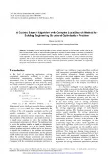
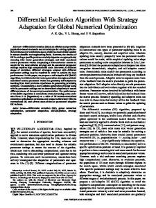
[15]. The population size parameter N P was set equal to approximation set size for each of the functions, i.e. 100, 150, and 800, respectively. For the constraint handling method, following parameters were chosen: θ = 0.3N P , β = 0.7N P , cp = 5, α1 = 0.8, α2 = 2.0, and Gc =0.2Gmax . C. Obtained Results For 30 runs on the test function suite [3] we obtained the IGD metric values given in Figure 1. The subfigures show evolution of the means and standard deviations of IGD metric values of the approximate sets obtained with the number of function evaluations (generations) for all test instances. For all functions, mean IGD value gradually improves with some deteriorations due to the multiobjective selection tradeoff differences in IGD and SPEA2 metrices. Sometimes the SPEA2 multiobjective selection metric used in our algorithm, assessed an approximation set differently to the IGD metric. While the SPEA2 metric seemed to improve the approximation sets and the standard deviation of the measured approximation sets was improving, their IGD metric assessment value got worse. This effect can be observed at ends of the optimization runs for functions UF2, UF3, UF4, R2 DTLZ3 M5, CF1, CF4, CF8, and CF10. Standard deviation also follows the mean IGD values given in Figure 1, except for the functions CF1 and WFG1. For function WFG1, standard deviation increases each time the local search is activated. For function CF1, the standard deviation follows the mean values of IGD, but starts to fluctuate more after nearly 0.1 IGD value is attained which again seems to be due to differences in selection metrices. The average IGD metric vales of the 30 final approximation sets obtained for each test problem are given in Table I. As seen from the assessment of results, the Pareto fronts of the unconstrained function instances were all approximated to the extent of IGD metric value being smaller than 0.38, except for the R2 DTLZ3 M5 and WFG1 M5 problems. The best approximated unconstrained functions seem to be UF1–UF4 and UF7. The constrained functions were all approximated to the extent of feasible region, with the exception of CF3 test problem. The IGD metric values of the remaining constrained test problems was below 0.2605 for CF1, CF2, CF4, and CF6–CF9. For test problem CF3, no feasible solution was obtained. The best attained approximation sets, i.e. those with minimal IGD metric values, are shown in Figure 2. As it was also evidenced from the Table I and Figure 1, it is clearly seen that the best attained function was UF4. For functions CF1 and CF2, many non-feasible solutions were found and therefore also, the evolution of their standard deviations for IGD metric in Figure 1 is fluctuating so much. The algorithm had most problems with the constrained test problem instances. For functions CF1 and CF3–CF7, there were only few non-dominated solutions in the approximation sets. For the functions CF8–CF10, there were more solutions in the approximation sets, but still quite sparse which again

TABLE I T HE AVERAGE IGD METRIC VALES OF THE 30 FINAL APPROXIMATION SETS OBTAINED AND

CPU TIME IN SECONDS USED FOR EACH TEST PROBLEM .

Function name IGD mean

IGD std

IGD best IGD worst CPU time

UF1

0.0770281 0.039379

0.055126 0.0880129

UF2

0.0283427 0.0313182 0.0173361 0.040226

7.17267

UF3

0.0935006 0.197951 0.0305453 0.168162

8.17833

UF4

0.0339266 0.00537072 0.0316247 0.035643

5.74567

UF5

0.167139 0.0895087 0.133012

0.237081

3.48233

UF6

0.126042

0.561753 0.0579174 0.589904

3.41167

UF7

0.024163 0.0223494 0.0198913 0.0427502

UF8

0.215834

0.121475 0.0989388 0.228895

16.6217 10.2383

UF9

0.14111

0.345356 0.0772668 0.332909

UF10

0.369857

0.65322

CF1

0.107736

0.195921 0.0581246 0.186248

CF2

0.0946079 0.294282

0.580852

0.037197

0.257011

1e+06

1e+06

6.206

6.818 28.1633 4.85267

CF3

1000000

CF4

0.152659

0.466596 0.0533448 0.301675

CF5

0.412756

0.590779 0.0963843 0.537761

4.598

CF6

0.147824

0.124723 0.0823086 0.186999

6.81233

CF7

0.26049

0.259938

CF8

0.176344

0.625776 0.0977472 0.420665

16.7807

CF9

0.127132

0.145787

0.108369

0.265246

13.4307

CF10

0.507051

1.19892

0.284772

0.811085

16.7113

R2 DTLZ2 M5 0.383041

0.11695

0.336664

0.418682

104.06

R2 DTLZ3 M5 943.352

551.654

745.167

1206.18

156.276

1.42433

1.83629

3.31374

170.543

WFG1 M5

1.9178

0

0.238279

4.434

0.170495

0.373809

3.574 4.08333

4.586

shows that the constrained function subset was much harder to solve than the unconstrained subset. The average CPU time used for each test problem was also measured. The function runs were performed in parallel, but each run was run in sequence, from random seeds taking values of 1 to 30. The average user mode CPU times for the processes of each optimization run are given in Table I. As seen from the results reported, optimization of test problems R2 DTLZ2 M5, R2 DTLZ3 M5, and WFG1 M5 take the most CPU time. All the remaining test problems optimizations finished below 30 seconds, i.e. less than 15 minutes for 30 runs of a test problem. The total execution time of the parallelized optimization and performance assessment with the IGD metric takes less than 4 hours on the system used. V. C ONCLUSIONS We have presented an algorithm for constrained multiobjective optimization. Its performance assessment was obtained using the test function suite from special session on multiobjective optimization at CEC 2009. On 23 test problems 30 runs are performed and results are assessed using the IGD metric. The results indicate that the approach used may be considered for constrained optimization as well the unconstrained multiobjective optimization. Future work could assemble in more instrumentation of the control parameters of the presented DECMOSA-SQP algorithm.

1.4 1.2 1 0.8 0.6 0.4 0.2 0

0.7 0.6 0.5 0.4 0.3 0.2 0.1 0

IGD mean for UF1 IGD standard deviation for UF1

0

500

1000

1500

2000

2500

0.6 0.4 0.2 0 0

500

1000

6

2000

2500

3000

1500

1.4 1.2 1 0.8 0.6 0.4 0.2 0

4

3

3

2

2

2000

2500

500

1000

2000

1000

3.5 3 2.5 2 1.5 1 0.5 0 2500

0

200

400

600

800

200

400

600

5 4.5 4 3.5 3 2.5 2 1.5 1 0.5 0

1000

1200

1400

1600

1800

50

100

150

800

1e+06

250

300

2000

2500

3000

150

500

1000

3 2 1 0 1000

1500

1400

1600

1800

2000

0

200

400

600

800

2000

2500

3000

200

250

300

350

400

0

50

100

1600

1800

2000

1500

2000

150

200

250

300

350

400

(l) R2 DTLZ3 M5 1.6 1.4 1.2 1 0.8 0.6 0.4 0.2 0

2500

IGD mean for CF2 IGD standard deviation for CF2

3000

0

500

1000

1500

2000

2500

3000

(o) CF2 IGD mean for CF5 IGD standard deviation for CF5

10

6 4 2 0 500

1000

1500

2000

2500

3000

0

500

1000

1500

9 8 7 6 5 4 3 2 1 0


0

500

1000

1500

2000

2500

3000

2500

3000


0

200

400

600

800

1000

1200

1400

1600

1800

2000

(u) CF8 12


2000

(r) CF5

(t) CF7

3

1400

8

(s) CF6 2.5

1200

IGD mean for R2_DTLZ3_M5 IGD standard deviation for R2_DTLZ3_M5

2500

12

0

3000

1000

(i) UF9


14 12 10 8 6 4 2 0


2500


(q) CF4

4

500

1200


(p) CF3 5

2000

0 100

5 4.5 4 3.5 3 2.5 2 1.5 1 0.5 0

0

6

3.5 3 2.5 2 1.5 1 0.5 0

(n) CF1

200000 1500

1000

1500

(f) UF6

500 50

0

400000

1000

1000

1000

350

600000

500

500

1500

0.45 0.4 0.35 0.3 0.25 0.2 0.15 0.1 0.05


0

0

(k) R2 DTLZ2 M5

200

3000

2000

(m) WFG1

800000

2500

IGD mean for R2_DTLZ2_M5 IGD standard deviation for R2_DTLZ2_M5

0

IGD mean for WFG1_M5 IGD standard deviation for WFG1_M5

0

2000

(h) UF8

(j) UF10 4 3.5 3 2.5 2 1.5 1 0.5 0

1500


0


2500

0 500

(g) UF7 16 14 12 10 8 6 4 2 0

2000


(e) UF5

1500

1500

1 0


0

1000

5

4

0 1000

500

6

1 500

0

(c) UF3


5

(d) UF4

0

1500

(b) UF2


0


1 0.8

(a) UF1 0.2 0.18 0.16 0.14 0.12 0.1 0.08 0.06 0.04 0.02 0

1.2



10

2

8

1.5

6

1

4 2

0.5 0

0 0

200

400

600

800

1000

(v) CF9

1200

1400

1600

1800

2000

0

200

400

600

800

1000

1200

1400

1600

1800

2000

(w) CF10

Fig. 1. Evolution of the means and standard deviations of IGD metric values of the approximate sets obtained with the generation number for all test instances.

1.2

1.2

UF1 approximation set UF1 Pareto front

1

0.8

0.6

0.6

0.4

0.4

0.2

0.2

0

0 0

0.2

0.4

0.6

0.8

1

0.4 0.2 0

1.2

0

0.2

0.4

0.6

0.8

1

1.2

0

0.2

0.4

(b) UF2 1


1


0.8 0.6

(a) UF1 1.2

1


1

0.8

1.2


0.8

0.8

0.6

0.8

1

(c) UF3 UF6 approximation set UF6 Pareto front

1 0.8

0.6

0.6

0.6 0.4

0.4

0.4

0.2

0.2 0

0.2

0 0

0.2

0.4

0.6

0.8

1

0

1.2

0

0.2

0.4

(d) UF4 UF7 approximation set UF7 Pareto front

1

1.2 1 0.8 0.6 0.4 0.2 0

0.8 0.6 0.4

0 0.2 0.4 0.6 0.8

0.2

1 1.2 1.4 1.6

(h) UF8

0 0.2

0.4

0.8

1

0

0.2

0.4

0.6

(e) UF5

1.2

0

0.6

0.6

0.8

1

0.8

1

1.2

(f) UF6 1.8 1.6 1.4 1.2 1 0.8 0.6 0.4 0.2 0

3 2 2.5 1 1.5 0 0.5

0

0.5

1

1.5

2

2.5

(i) UF9

0.8 1 0.40.6 0 0.2

2 1.61.8 1.21.4

1.2

(g) UF7 1 1.2 1 0.8 0.6 0.4 0.2 0 0

1.2

CF1 approximation set CF1 Pareto front

0.8

0.2

0.4

0.6

0.4 0 0.2

0.8

1 1.2 (j) UF10

0.6 0.8


1 0.8

0.6

0.6

1.4 1 1.2

0.4

0.4

0.2

0.2

0

0 0

0.2

0.4

0.6

0.8

1

0

0.2

0.4

(k) CF1 1.2

1.1 1 0.9 0.8 0.7 0.6 0.5 0.4 0.3 0.2 0.1


1 0.8 0.6 0.4 0.2 0 0

0.2

0.4

0.6

0.8

1

1.2

1.2

1.1 1 0.9 0.8 0.7 0.6 0.5 0.4 0.3 0.2 0.1


0

0.2

0.4

(m) CF3

0.6

1.2

0.8

1

0


0.8

0.6

0.6

3 2.5 2 1.5 1 0.5 0

0.4

0.4

0

0.2

0.2

0

0.2

0.4

0.5

1

0 0

0.2

0.4

0.6

0.8

1

1.2

1.4

1.6

0

0.2

(p) CF6

0.5

0.6

1.2

0.6

0.8

1

1.2

1.4

1.6

0.8

1

1.5

2

2.5

3

3.5

(r) CF8

3 2 2.5 1 1.5 0 0.5

1.2

(q) CF7

6 5 4 3 2 1 0 0

0.4

1

(o) CF5

0.8

1

0.8


(n) CF4 CF6 approximation set CF6 Pareto front

1

0.6

(l) CF2

1

1.5

2

2.5

3

(s) CF9

Fig. 2.

0

0.5

1

1.5

2

2.5

1.2 1 0.8 0.6 0.4 0.2 0 0

0.2

0.4

0.6

0.8

1

1.2

(t) CF10

30 35 20 25 10 15 0 5

Pareto front and best attained approximation set for all test instances.

ACKNOWLEDGMENT We thank the authors of CfSQP for providing us with the academic license of their software. R EFERENCES [1] J. Knowles, L. Thiele, and E. Zitzler, “A Tutorial on the Performance Assessment of Stochastic Multiobjective Optimizers,” Computer Engineering and Networks Laboratory (TIK), ETH Zurich, Switzerland,” 214, Feb. 2006, revised version. [2] K. Deb, Multi-Objective Optimization using Evolutionary Algorithms. Chichester, UK: John Wiley & Sons, 2001, ISBN 0-471-87339-X. [3] Q. Zhang, A. Zhou, S. Zhao, P. N. Suganthan, W. Liu, and S. Tiwari, “Multiobjective optimization Test Instances for the CEC 2009 Special Session and Competition,” Department of Computing and Electronic

Systems and School of Electrical and Electronic Engineering and Department of Mechanical Engineering, University of Essex, Colchester, C04, 3SQ, UK and Nanyang Technological University, 50 Nanyang Avenue, Singapore and Clemson University, Clemson, SC 29634, US, Tech. Rep. CES-487, 2007. ˇ [4] J. Brest, A. Zamuda, B. Boˇsković, and V. Zumer, “An Analysis of the Control Parameters Adaptation in DE,” in Advances in Differential Evolution, Studies in Computational Intelligence, U. K. Chakraborty, Ed. Springer, 2008, vol. 143, pp. 89–110. ˇ [5] A. Zamuda, J. Brest, B. Boˇsković, and V. Zumer, “Differential Evolution for Multiobjective Optimization with Self Adaptation,” in The 2007 IEEE Congress on Evolutionary Computation CEC 2007. IEEE Press, 2007, pp. 3617–3624, DOI: 10.1109/CEC.2007.4424941. [6] C. T. Lawrence, J. L. Zhou, and A. L. Tits, “User’s Guide for CFSQP Version 2.5: A C Code for Solving (Large Scale) Constrained Nonlinear (Minimax) Optimization Problems, Generating Iterates Satisfying

[7]

[8]

[9]

[10]

[11]

[12]

[13]

[14]

[15] [16]

[17] [18]

[19]

[20]

[21]

[22]

[23]

[24]

All Inequality Constraints,” Institute for Systems Research, University of Maryland, College Park, MD 20742, Tech. Rep., 1997, TR-94-16r1. T. Robiˇc and B. Filipiˇc, “DEMO: Differential Evolution for Multiobjective Optimization,” in Proceedings of the Third International Conference on Evolutionary Multi-Criterion Optimization – EMO 2005, ser. Lecture Notes in Computer Science, vol. 3410. Springer, 2005, pp. 520–533. T. Tuˇsar and B. Filipiˇc, “Differential Evolution versus Genetic Algorithms in Multiobjective Optimization,” in Proceedings of the Fourth International Conference on Evolutionary Multi-Criterion Optimization – EMO 2007, ser. Lecture Notes in Computer Science, vol. 4403. Springer, 2007, pp. 257–271. ˇ ˇ A. Zamuda, J. Brest, B. Boˇsković, and V. Zumer, “Studija samoprilagajanja krmilnih parametrov pri algoritmu DEMOwSA,” Elektrotehniˇski vestnik, vol. 75, no. 4, pp. 223–228, 2008. R. Storn and K. Price, “Differential Evolution – A Simple and Efficient Heuristic for Global Optimization over Continuous Spaces,” Journal of Global Optimization, vol. 11, pp. 341–359, 1997. H. A. Abbass, “The self-adaptive Pareto differential evolution algorithm,” in Proceedings of the 2002 Congress on Evolutionary Computation, 2002 (CEC ’02), vol. 1, May 2002, pp. 831–836. K. Deb, S. Agrawal, A. Pratab, and T. Meyarivan, “A Fast Elitist NonDominated Sorting Genetic Algorithm for Multi-Objective Optimization: NSGA-II,” in Proceedings of the Parallel Problem Solving from Nature VI Conference, M. Schoenauer, K. Deb, G. Rudolph, X. Yao, E. Lutton, J. J. Merelo, and H.-P. Schwefel, Eds. Paris, France: Springer. Lecture Notes in Computer Science No. 1917, 2000, pp. 849–858. E. Zitzler, M. Laumanns, and L. Thiele, “SPEA2: Improving the Strength Pareto Evolutionary Algorithm for Multiobjective Optimization,” in Evolutionary Methods for Design Optimization and Control with Applications to Industrial Problems, K. C. Giannakoglou, D. T. Tsahalis, J. Périaux, K. D. Papailiou, and T. Fogarty, Eds. Athens, Greece: International Center for Numerical Methods in Engineering (CIMNE), 2001, pp. 95–100. E. Zitzler and S. Künzli, “Indicator-Based Selection in Multiobjective Search,” in Parallel Problem Solving from Nature (PPSN VIII), X. Yao et al., Eds. Berlin, Germany: Springer-Verlag, 2004, pp. 832–842. H.-G. Beyer and H.-P. Schwefel, “Evolution strategies — A comprehensive introduction,” Natural Computing, vol. 1, pp. 3–52, 2002. T. Bäck, Evolutionary Algorithms in Theory and Practice: Evolution Strategies, Evolutionary Programming, Genetic Algorithms. New York: Oxford University Press, 1996. H.-P. Schwefel, Evolution and Optimum Seeking, ser. Sixth-Generation Computer Technology. New York: Wiley Interscience, 1995. ˇ J. Brest, S. Greiner, B. Boˇsković, M. Mernik, and V. Zumer, “SelfAdapting Control Parameters in Differential Evolution: A Comparative Study on Numerical Benchmark Problems,” IEEE Transactions on Evolutionary Computation, vol. 10, no. 6, pp. 646–657, 2006, DOI: 10.1109/TEVC.2006.872133. ˇ J. Brest, V. Zumer, and M. S. Mauˇcec, “Self-adaptive Differential Evolution Algorithm in Constrained Real-Parameter Optimization,” in The 2006 IEEE Congress on Evolutionary Computation CEC 2006. IEEE Press, 2006, pp. 919–926. ˇ A. Zamuda, J. Brest, B. Boˇsković, and V. Zumer, “Large Scale Global Optimization Using Differential Evolution with Self Adaptation and Cooperative Co-evolution,” in 2008 IEEE World Congress on Computational Intelligence. IEEE Press, 2008, pp. 3719–3726. J. Brest and M. S. Mauˇcec, “Population Size Reduction for the Differential Evolution Algorithm,” Applied Intelligence, vol. 29, no. 3, pp. 228–247, 2008, DOI: 10.1007/s10489-007-0091-x. V. L. Huang, A. K. Qin, K. Deb, E. Zitzler, P. N. Suganthan, J. J. Liang, M. Preuss, and S. Huband, “Problem Definitions for Performance Assessment & Competition on Multi-objective Optimization Algorithms,” Nanyang Technological University et. al., Singapore, Tech. Rep. TR07-01, 2007. K. Deb, L. Thiele, M. Laumanns, and E. Zitzler, “Scalable MultiObjective Optimization Test Problems,” in Congress on Evolutionary Computation (CEC’2002), vol. 1. Piscataway, New Jersey: IEEE Service Center, May 2002, pp. 825–830. S. Huband, P. Hingston, L. Barone, and L. While, “A Review of Multiobjective Test Problems and a Scalable Test Problem Toolkit,” IEEE Transactions on Evolutionary Computation, vol. 10, no. 5, pp. 477–506, October 2006.

[25] P. Boggs and J. Tolle, “Sequential quadratic programming for largescale nonlinear optimization,” Journal of Computational and Applied Mathematics, vol. 124, no. 1-2, pp. 123–137, 2000, DOI: 10.1016/S0377-0427(00)00429-5. ˇ [26] J. Brest, B. Boˇsković, S. Greiner, V. Zumer, and M. S. Mauˇcec, “Performance comparison of self-adaptive and adaptive differential evolution algorithms,” Soft Computing - A Fusion of Foundations, Methodologies and Applications, vol. 11, no. 7, pp. 617–629, 2007, DOI: 10.1007/s00500-006-0124-0. [27] R. Storn and K. Price, “Differential Evolution - a simple and efficient adaptive scheme for global optimization over continuous spaces,” Berkeley, CA, Tech. Rep. TR-95-012, 1995. [28] K. V. Price, R. M. Storn, and J. A. Lampinen, Differential Evolution: A Practical Approach to Global Optimization, ser. Natural Computing Series, G. Rozenberg, T. Bäck, A. E. Eiben, J. N. Kok, and H. P. Spaink, Eds. Berlin, Germany: Springer-Verlag, 2005. [29] V. Feoktistov, Differential Evolution: In Search of Solutions (Springer Optimization and Its Applications). Secaucus, NJ, USA: SpringerVerlag New York, Inc., 2006. [30] H.-Y. Fan and J. Lampinen, “A Trigonometric Mutation Operation to Differential Evolution,” Journal of Global Optimization, vol. 27, no. 1, pp. 105–129, 2003. [31] M. M. Ali and A. Törn, “Population set-based global optimization algorithms: some modifications and numerical studies,” Comput. Oper. Res., vol. 31, no. 10, pp. 1703–1725, 2004. [32] H. A. Abbass, R. Sarker, and C. Newton, “PDE: A Pareto-frontier Differential Evolution Approach for Multi-objective Optimization Problems,” in Proceedings of the Congress on Evolutionary Computation 2001 (CEC’2001), vol. 2. Piscataway, New Jersey: IEEE Service Center, May 2001, pp. 971–978. ˇ [33] T. Tuˇsar, P. Koroˇsec, G. Papa, B. Filipiˇc, and J. Silc, “A comparative study of stochastic optimization methods in electric motor design,” Applied Intelligence, vol. 2, no. 27, pp. 101–111, 2007, DOI 10.1007/s10489-006-0022-2. [34] A. E. Eiben and J. E. Smith, Introduction to Evolutionary Computing (Natural Computing Series). Springer, November 2003. [35] J. Holland, Adaptation In Natural and Artificial Systems. Ann Arbor: The University of Michigan Press, 1975. [36] X. Yao, Y. Liu, and G. Lin, “Evolutionary Programming Made Faster,” IEEE Transactions on Evolutionary Computation, vol. 3, no. 2, pp. 82–102, 1999. [37] Y. Liu, X. Yao, Q. Zhao, and T. Higuchi, “Scaling Up Fast Evolutionary Programming with Cooperative Coevolution,” in Proceedings of the 2001 Congress on Evolutionary Computation CEC 2001. COEX, World Trade Center, 159 Samseong-dong, Gangnam-gu, Seoul, Korea: IEEE Press, 27-30 2001, pp. 1101–1108. [38] A. E. Eiben, R. Hinterding, and Z. Michalewicz, “Parameter Control in Evolutionary Algorithms,” IEEE Trans. on Evolutionary Computation, vol. 3, no. 2, pp. 124–141, 1999. [39] J. Liu and J. Lampinen, “A Fuzzy Adaptive Differential Evolution Algorithm,” Soft Comput., vol. 9, no. 6, pp. 448–462, 2005. [40] J. Teo, “Exploring dynamic self-adaptive populations in differential evolution,” Soft Computing - A Fusion of Foundations, Methodologies and Applications, vol. 10, no. 8, pp. 673–686, 2006. [41] G. V. Reklaitis, A. Ravindran, and K. M. Ragsdell, Engineering Optimization: Methods and Applications. Wiley-Interscience, 1983. [42] Z. Michalewicz and M. Schoenauer, “Evolutionary Algorithms for Constrained Parameter Optimization Problems,” Evolutionary Computation, vol. 4, no. 1, pp. 1–32, 1996. [43] S. Koziel and Z. Michalewicz, “Evolutionary Algorithms, Homomorphous Mappings, and Constrained Parameter Optimization.” Evolutionary Computation, vol. 7, no. 1, pp. 19–44, 1999. [44] Z. Michalewicz and D. B. Fogel, How to Solve It: Modern Heuristics. Berlin: Springer, 2000. [45] C. Coello Coello, “Theoretical and numerical constraint-handling techniques used with evolutionary algorithms: a survey of the state of the art,” Computer Methods in Applied Mechanics and Engineering, vol. 191, no. 11-12, pp. 1245–1287, 2002. [46] J. Brest, “Constrained Real-Parameter Optimization with ǫ-SelfAdaptive Differential Evolution,” in Constraint-Handling in Evolutionary Optimization. Springer, accepted. [47] T. Takahama, S. Sakai, and N. Iwane, “Solving Nonlinear Constrained Optimization Problems by the ǫ Constrained Differential Evolution,” Systems, Man and Cybernetics, 2006. SMC ’06. IEEE International Conference on, vol. 3, pp. 2322–2327, 8-11 Oct. 2006.