Local Search for Flowshops with Setup Times and Blocking Constraints

Twenty-Eighth International Conference on Automated Planning and Scheduling (ICAPS 2018)

Local Search for Flowshops with Setup Times and Blocking Constraints Vahid Riahi, M. A. Hakim Newton, Kaile Su, Abdul Sattar Institute for Integrated and Intelligent Systems (IIIS), Griffith University, Australia vahid.riahi@griffithuni.edu.au, {mahakim.newton, k.su, a.sattar}@griffith.edu.au

pendent setup time (SDST) si[k][k+1] is neither part of pi[k] nor of pi[k+1] , since it depends on two successive jobs in the permutation. SDSTs are important because these are present in about 70% of industrial activities (Dudek, Smith, and Panwalkar 1974). For example, in the paper cutting industry, the cutting machines need adjustment before starting a different type of cutting batch. In the painting industry, cleaning must be performed before changing the painting colors. More examples could be found in the survey by (Allahverdi 2015). In another PFSP variant known as limited-buffer PFSP, each buffer has a limited capacity. In yet another variant known as blocking PFSP, each buffer capacity is zero. This means a job might have to stay at the machine that processed it and might thus block the machine. Formally, a machine i < m cannot start processing an available job [k] until machine i + 1 starts processing job [k − 1]. This constraint in the blocking PFSP is known as Release when Starting Blocking (RSb). Blocking PFSPs have been studied by (Ribas and Companys 2015; Tasgetiren et al. 2017a). Besides the traditional RSb blocking, there exists a special blocking named Release when Completing Blocking (RCb)1 (Martinez de La Piedra 2005), where a machine i < m cannot start processing an available job [k] until job [k−1] leaves machine i+1. RCb blocking is seen in real-life industries such as waste treatment and aeronautics parts fabrication industries (Martinez de La Piedra 2005). In waste treatment industries, wastes from each cargo is unloaded to a tank and then the wastes flow to the blender. The tank is not available for further unloading until the blending is finished and the blended wastes completely leave the blender. Despite existence of several PFSP variants, significant modelling gaps still exist when real-world industrial applications are considered. In this research, we study PFSPs with both SDSTs and mixed blocking constraints (RSb and RCb) considering makespan minimisation as the objective. For each machine, our model allows SDST for the next job to be overlapping with the blocking or idle time of the machine for the current job. Our motivation comes from real-life applications of this PFSP variant, for example, from the cider industry. The cider production process consists of seven stages that include pressing and fermentation. Workers must set up a machine with the right setting and ingredients before start-

Abstract Permutation flowshop scheduling problem (PFSP) is a classical combinatorial optimisation problem. There exist variants of PFSP to capture different realistic scenarios, but significant modelling gaps still remain with respect to real-world industrial applications such as the cider production line. In this paper, we propose a new PFSP variant that adequately models both overlapable sequence-dependent setup times (SDST) and mixed blocking constraints. We propose a computational model for makespan minimisation of the new PFSP variant and show that the time complexity is NP Hard. We then develop a constraint-guided local search algorithm that uses a new intensifying restart technique along with variable neighbourhood descent and greedy selection. The experimental study indicates that the proposed algorithm, on a set of wellknown benchmark instances, significantly outperforms the state-of-the-art search algorithms for PFSP.

Introduction Permutation Flowshop Scheduling Problems (PFSP) are one of the most well-known machine scheduling problems. A PFSP has a sequence of m machines. Each machine i has a buffer i of a given capacity ci before the machine to hold the arriving jobs. Each buffer is a first-come-first-serve queuing system. After the current job at machine i is completed, the next job j from buffer i is removed from the buffer and is then processed by machine i taking given processing time pij . Each processed job j from machine i then goes to buffer i + 1. The PFSP problem is to find a permutation π of a given set of n jobs such that when the jobs are placed in buffer 1 exactly in the permutation order and the flowshop starts running, then the resulting makespan of processing all jobs by all machines is minimised. Assuming [k] denotes the kth job in the permutation π, the makespan is the time point when the last job leaves the last machine. In a typical PFSP, each buffer has an infinite capacity and jobs can stay in each buffer for an unlimited period of time. There exist variants of PFSP to capture different realistic scenarios, where each variant poses its own scheduling challenges. In one PFSP variant, each machine i after processing job [k] needs sequence dependent si[k][k+1] time to be set up before processing next job [k + 1]. Note that the sequence dec 2018, Association for the Advancement of Artificial Copyright  Intelligence (www.aaai.org). All rights reserved.

1

199

Should be renamed as Release when Leaving Blocking (RLb)

RSb RCb

RSb RCb

m 1 2 3 m 1 2 3

1

1

3

1

blocking time 3 10

2 5

1

3 2

2 1 1

setup time

t

3 3

2 5

can be performed as soon as the machine finish the current job regardless of the state that the current job is still on the machine or not. Clearly, setup operations could be deferred if there is a slack period before starting processing the next job. However, such deferral does not pose any further computational challenge. Figure 1 bottom shows the case when SDSTs are overlapable and blocking constraints are mixed. Sometimes blocking or idle times could be larger than SDSTs and sometimes it is other way around. It is worth noting that in the proposed PFSP variant, all other common flowshop assumptions (Baker 1974) still apply: (1) all jobs are independent and available beforehand; (2) machines are always available and never break down; (3) jobs put on machines are processed without interruptions and cannot be taken off until the operations to be performed are completed by the respective machines.

idle time

3 2

2

10

t

Figure 1: PFSPs with top) RSb and RCb constraints bottom) overlapable SDSTs, and RSb and RCb constraints ing processing for a specific type of apple juice (thus SDSTs). Moreover, apples of a job must stay in the stock until the washing machine is available (RSb constraint) and the next job must stay at the pressing stage until the current job leaves the fermentation stage (RCb constraint). To the best of our knowledge, there is no available research on PFSPs with both overlapable SDSTs and mixed blocking constraints, although this variant has real-world industrial applications. In this paper, we propose a computational model for PFSPs with overlapable SDSTs and mixed blocking constraints (RSb and RCb) and next show that minimisation of the makespan of the PFSP variant is NP Hard. In order to solve the studied problem, we present a very efficient constraint-guided local search algorithm that uses a new intensifying restart along with variable neighbourhood descent and greedy selection. For the proposed algorithm, we also provide a speed-up method that is similar to the one developed by (Li, Wang, and Wu 2009). The proposed algorithm is tested on a set of benchmark instances and found to be significantly outperforming adapted state-of-the-art local search algorithms for closely related problems. In the rest of the paper, we propose the PFSP variant, describe the search algorithm, present the experimental results, review the related work, and present the conclusions.

Computational Formulas Assume pij be the given processing time for job j on machine i and sijj  be the SDST of machine i after finishing job j and before starting job j  = j. Given a permutation π of n jobs, also assume Si[k] , Ci[k] , and Li[k] respectively denote the starting, completion, and leaving time points for i[k] processing job [k] on machine i. Moreover, assume S  i[k] respectively denote the SDST starting and comand C pletion time points before job [k] on machine i. Finally, assume Bi ∈ {RSb, RCb} be the type of blocking constraint between machines i and i + 1 since ci+1 is zero. Given a permutation π of n jobs, the makespan Cπ = Cm[n] is the completion time of job [n] on machine m. Makespan computation for PFSPs with overlapable SDSTs and RSb and RCb blocking constraints is far from being straightforward. We define required formulas below. 1. Ci[k] = Si[k] + pi[k] ∀i ∈ [1, m], ∀k ∈ [1, n] 2. Li[k] = S(i+1)[k] ∀i ∈ [1, m − 1], ∀k ∈ [1, n] Lm[k] = Cm[k] ∀k ∈ [1, n] i[k] = Ci[k−1] ∀i ∈ [1, m], ∀k ∈ [2, n] 3. S i[k] + si[k−1][k] ∀i ∈ [1, m], k ∈ [2, n]  i[k] = S 4. C 5. S1[1] = 0, Si[1] = C(i−1)[1] ∀i ∈ [2, m]  1[k] , S2[k−1] ) if B1 = RSb ∀k ∈ [2, n] S1[k] = max(C

Proposed Problem Model Under RSb, a machine cannot start processing a job until the next machine starts processing the previous job. In Figure 1 top, machine 1 starts job 2 and job 3 when machine 2 starts job 1 and job 2 respectively. Under RCb, a machine cannot start processing a job until the previous job leaves the next machine. In Figure 1 top, machine 2 starts job 2 and job 3 when job 1 and job 2 leave machine 3 respectively. RCb constraints are more stringent than RSb constraints Machine setup times could be part of the processing times or could be separate. In the latter case, for a job [k], the setup time period of machine i can be considered for overlapping with the idle or blocking time of machine i − 1 and/or can also be considered to be dependent on the job [k − 1] on machine i (SDST). Considering our motivation from the cider industry, in this paper, we adopt overlapable SDSTs. In our proposed model for PFSPs with overlapable SDSTs and mixed RSb and RCb blocking constraints, we make one important assumption: setup operations for the next job

 1[k] , L2[k−1] ) if B1 = RCb ∀k ∈ [2, n] S1[k] = max(C  i[k] , S(i+1)[k−1] ) Si[k] = max(C(i−1)[k] , C if Bi = RSb ∀i ∈ [2, m − 1], ∀k ∈ [2, n]  i[k] , L(i+1)[k−1] ) Si[k] = max(C(i−1)[k] , C if Bi = RCb ∀i ∈ [2, m − 1], ∀k ∈ [2, n]  m[k] ) ∀k ∈ [2, n] Sm[k] = max(C(m−1)[k] , C

Formula 1 above computes completion time point of each job on each machine by adding the processing time period to the starting time point. Formula 2 computes the leaving time point of each job from each machine. A job leaves the last machine as soon as it is finished; otherwise the leaving time point from the current machine is the same as the starting time point of the job on the next machine. Formula 3 computes SDST starting point for each job on a given machine from the completion time point of the previous job on

200

the same machine. Formula 4 then adds SDST period to the SDST starting time point to obtain SDST completion time point. Formula 5 computes the starting time point of each job on each machine. There is no SDST for the first machine and there is no blocking constraint after the last machine. For other machines, the starting time of a job is computed i) from its completion on the previous machine, ii) from the completion of the SDST period on the same machine, and iii) depending on the RSB or RCB constraint, respectively from the starting or leaving time point of the previous job on the next machine.

can speed up the makespan calculation significantly (up to 40-50% time saving), particularly in the large instances having large numbers of jobs (Li, Wang, and Wu 2009).

Time Complexity We now provide the following lemma to show the time complexity of the proposed PFSP variant. Lemma 1 Makespan minimisation of PSFPs with overlapable SDSTs and mixed RSB and RCb blocking constraints are NP Hard when m > 4. Proof: Consider the particular instance where SDSTs are all set to zero. Thus, the RSb-RCb-SDST-PFSP problem is transformed to an RSb-RCb-PFSP problem that is known to be NP Hard when m>4 (Martinez et al. 2006).

An Illustrative Example Consider the example shown in Figure 1 bottom, where the PFSP with overlapable SDSTs and mixed blocking constraints has 3 machines and 3 jobs. The processing time for each job j on each machine i is shown in the matrix |pij | below. Also, the SDST for each pair of jobs j = j  on machine i is shown in the matrix |sijj  | below. The blocking constraints are B = RSb, RCb. 2 2 1 |pij | = 1 1 2 1 1 2

- 2 2 |sijj  | = 1 - 1 1 2 -

- 2 3 2 - 2 3 2 -

Proposed Search Algorithm For the proposed PFSP variant, we develop an effective constraint-guided local search (CGLS) algorithm. Three variants CGLS1, CGLS2, and CGLS3 of the proposed algorithms are shown in Algorithm 1. We design a variable neighbourhood descent (VND) method for local search in all variants. For initial solution construction, we use two heuristics NNEH and SNEH, which are developed based on the NEH heuristic (Nawaz, Enscore, and Ham 1983). Moreover, for CGLS3, we use an intensifying restart method IR. We describe the NNEH, SNEH, IR and VND in details.

- 3 2 2 - 2 1 3 -

 and C  values for the permutation Below we show S, C, L, S, of jobs π = 1, 2, 3, but, not in the order of computation. S1[1] = 0

C1[1] = S1[1] + p1[1] = 2

L1[1] = S2[1] = 2

S2[1] = C1[1] = 2

C2[1] = S2[1] + p2[1] = 4

S3[1] = C2[1] = 4 1[2] = C1[1] = 2 S 2[2] = C2[1] = 4 S 3[2] = C3[1] = 5 S

C3[1] = S3[1] + p3[1] = 5  1[2] = C  2[2] = C  3[2] C

 1[2] , S2[1] ) = 4 S1[2] = max(C  2[2] , L3[1] ) = 6 S2[2] = max(C1[2] , C  3[2] ) = 8 S3[2] = max(C2[2] , C L1[2] = S2[2] = 6 1[3] = C1[2] = 5 S 2[3] = C2[2] = 7 S 3[3] = C3[2] = 10 S

L1[3] = S2[3] = 10

L3[1] = C3[1] = 5 1[2] + s1[1][2] = 4 S 2[2] + s2[1][2] = 6 S 3[2] + s3[1][2] = 8 =S

Algorithm 1: CGLS1 or CGLS2 or CGLS3 1 2

C1[2] = S1[2] + p1[2] = 5

3

C2[2] = S2[2] + p2[2] = 7

4

C3[2] = S3[2] + p3[2] = 10

L2[2] = S3[2] = 8

 1[3] , S2[2] ) = 6 S1[3] = max(C  2[3] , L3[2] ) = 10 S2[3] = max(C1[3] , C  3[3] ) = 12 S3[3] = max(C2[3] , C

L2[1] = S3[1] = 4

 1[3] C  2[3] C

5

L3[2] = C3[2] = 10 1[3] + s1[2][3] = 6 =S 2[3] + s2[2][3] = 9 =S

 3[3] = S 3[3] + s3[2][3] = 12 C

L2[3] = S3[3] = 12

π ∗ ← VND(NNEH() or SNEH() or SNEH()) while not timeout do π ← VND(NNEH() or SNEH() or IR(π ∗ )) if Cπ < Cπ∗ then π ∗ ← π // update best return π ∗ // best solution so far

Processing Times in Job Sorting for NNEH

C1[3] = S1[3] + p1[3] = 7

NEH (Nawaz, Enscore, and Ham 1983) is a very well-known greedy constructive heuristic for PFSP. Assuming O(n3 m) m wj = i=1 pij , NEH first sorts jobs on the non-increasing order of wj s to obtain a permutation π o . Let πk denote a permutation of k jobs and thus represent a partial solution. Starting from π0 , in each iteration k, NEH then obtains k +1 permutations πk+1 by inserting job [k] of π o in all positions of πk . NEH then selects the πk+1 with the minimum Cπk+1 to be used in the next iteration k + 1. Sometimes NEH when adapted to other PFSP variants outperform the original NEH. One such NEH variant (let the name be NEH-Raj) (Rajendran 1993) for typical PFSPs uses m the non-decreasing order of wj = i=1 (m − i + 1) × pij to sort the jobs to obtain π o and thus gives more priorities to jobs with smaller processing times on earlier machines than jobs with larger processing times. Another variant NEH-WPT (Wang, Pan, andTasgetiren 2011) uses the m non-decreasing order of wj = i=1 pij to sort the jobs in PFSPs with RSb blocking constraints. The intuition is that the jobs with higher total processing times may cause to

C2[3] = S2[3] + p2[3] = 11 3[3] + p3[3] = 14 C3[3] = S L3[3] = C3[3] = 14

Speed-Up Method Given a permutation π of n jobs to be scheduled on m machines, computing Cπ from scratch requires O(nm) times. Now, assume two permutations π and π  such that first n jobs are the same in both π and π  . Therefore, for both π and π  , Ci,[k] s are the same for k ≤ n . We need not calculate these completion time points for π  , if those are already known for π. We only need to compute the completion time points for the subsequent n − n jobs in π  . This speedup is important for time performance of a local search algorithm. Local search algorithms typically evaluate a large number of potential solutions before moving from the current solution to the next solution and these current and potential solution permutations very often differ from each other by a single insertion or swap move. Using such techniques, we

201

πs

2 3 5 1 4

3 2 5 1 4

3 4 2 5 1

3 4 2 1 5

tain π 2 = 3, 4, 2, 5, 1. Then, π 2 and π t differ at the fourth position. To match at that position, we can remove 1 from π 2 and insert before 5 to obtain π t = 3, 4, 2, 5, 1. In this way, the path relinking procedure shown in Algorithm 2 visits the intermediate solutions that share properties with π s and π t . Path relinking returns the intermediate solution with the least makespan.

πt

Figure 2: Path relinking procedure using insertion. block the successive jobs and to yield larger blocking times than the jobs with less total processing times. Yet another variant NNEH (Riahi et al. 2017) uses the non-decreasing m order of wj = i=1 [γ × (m − i + 1) × pij + (1 − γ) × pij ] to sort the jobs in PFSPs with mixed blocking constraints. Thus, NNEH combines NEH-Raj with NEH-WPT but is shown to have performed the best when γ = 0.1 i.e. when more weight is put on NEH-WPT than NEH-Raj. For CGLS1, we use the NNEH. However, instead of using just γ = 0.1, in each iteration of Algorithm 1, we use a randomly generated γ. A random γ produces a different initial solution in each iteration and ensures search diversity. Note that this option does not use SDSTs in solution construction.

Algorithm 2: Path relinking using insertion 1 2 3 4 5 6 7 8 9

Let π s and π t be the starting and target solutions. Cπ∗ = ∞ where π ∗ is the best intermediate solution. π m = π s // start from π s to visit intermediate solutions. for k = 1 to n do if π m and π t differ at position k then Assume j = job [k] in the target solution π t . Remove j from π m and insert at position k. if Cπm < Cπ∗ then let π ∗ = π m . return π ∗ as the output solution

Selection of π s and π t and the operator to be used (e.g. insertion) affect the performance of path relinking. In population based search, two solutions from the current populations are used. In this work, we use the best solution found so far (hence intensifying) as π s because path relinking has been observed to be performing better when starts from the better solution (Ribeiro, Uchoa, and Werneck 2002). For π t , a completely random solution is generated (hence diversifying). For the operator, we could use swap instead of insertion, but to keep the restart procedure somewhat consistent with the insertion-based construction algorithms NNEH and SNEH, we use insertion.

Setup Times in Job Sorting for SNEH For CGLS2 and CGLS3, we develop SNEH to incorporate SDSTs with NNEH. First, we define (sequence independent) n,j  =j average setup time sij = j  =1 (sijj  +sij  j )/(2n−2) for m job j on machine i. Then, we redefine wj = i=1 [β ×sij + (1 − β) × pij ] and use the non-decreasing order of wj s to sort the jobs. Notice that β is to balance the relative weight of setup time and processing time associated with job j on machine i. We prefer NEH-WPT to NEH-Raj in redefining wj since NNEH performs better with γ = 0.1, meaning NEH-WPT is more prominent than NEH-Raj. Like NEHWPT, We choose the non-decreasing order of wj because scheduling jobs with higher wj will tend to delay scheduling of subsequent jobs. We will later empirically study the effect of β values, but for now, it is sufficient to mention that no dominating β is observed and hence we choose a random β value in each iteration of Algorithm 1.

Constraint Guided Selection for VND Local search moves from one solution to another in quest of a better solution in each iteration. In this process, the neighbourhood operators used to generate the potential solutions from the current solution play a crucial role. Insertion and swap operators have been used widely when solutions are permutations e.g. in flowshops. In insertion, typically a randomly selected job is removed from the current solution and then reinserted in all possible positions to obtain the potential solutions. In swap, a randomly selected job is swapped with all jobs in the current solution to obtain the potential solutions. Notice that the job selection in these operators is done mostly randomly e.g. in algorithms by (Riahi and Kazemi 2016; Ruiz and St¨utzle 2008). In this paper, instead of random selection, we propose a constraint-guided greedy job selection approach for insertion and swap. Algorithm 3 presents our proposed insertion procedure GI. First, jobs are arranged in the non-increasing order of the total blocking time each job caused. Under blocking constraints, machines are blocked with the current jobs until subsequent machines are available. We can associate this blocking period of the machine to the job which it is currently holding. Given a solution π, each job [k] has the m−1 (R(i+1)[k] − Ci[k] ) where total blocking B[k] = i R(i+1)[k] = S(i+1)[k] if Bi = RSb or R(i+1)[k] = L(i+1)[k] if Bi = RCb. According to our greedy heuristic, the job

Path Relinking in Intensifying Restart IR For search diversity, CGLS1 and CGLS2 respectively use NNEH and SNEH (with random γ and β) as restart in each iteration. In these restart methods, there is no intensification towards the best solution found so far. We design a new intensifying restart method IR for CGLS3. We use the path relinking procedure (Glover 1997) to get a combination of the best solution found so far and a completely randomly generated solution. Path relinking is usually used in population based local search algorithms to diversify the search. For the first time, we use path relinking in a restarting strategy to achieve intensification within the diversification process. Assume π s = 2, 3, 5, 1, 4 and π t = 3, 4, 2, 1, 5 in Figure 2 are starting and target solutions respectively. When compared lexicographically, π s and π t differ in the first position. To match at that position, we can remove 3 from π s and insert before 2 and will thus get π 1 = 3, 2, 5, 1, 4. Next, π 1 and π t differ at the second position. To match at that position, we can remove 4 from π 1 and insert before 2 to ob-

202

[k] that causes the most total blocking B[k] should be selected for removal and reinsertion. Our motivation to do this is to fix the most problematic part of the current solution. For space constraints, we do not show the greedy swap GS, random insert RI, and random swap RS procedures, since these could be obvious given the pseudocode of GI.

PFSP instances are made up of 12 groups each comprising 10 instances of the same problem size. The problem sizes for the groups in terms of n × m combinations are: {20, 50, 100} × {5, 10, 20}, {200} × {10, 20} and {500 × 20}. In those instances, the job processing times pij s are uniformly distributed in the range of [1, 100). To add SDSTs to the 120 instances, (Ruiz, Maroto, and Alcaraz 2005) obtained four scenarios by generating sijj  uniformly randomly in the ranges of [1, 10), [1, 50), [1, 100) and [1, 125) and named these scenarios as SDST10, SDST50, SDST100 and SDST125, respectively. These scenarios allow us to see the effect of having SDSTs larger and smaller than processing times. To further add blocking constraints, in this work, we consider three scenarios: RSbOnly scenario where blocking constraints are all RSB, RCbOnly scenario where blocking constraints are all RCb, and RSb-RCb scenario where RSb and RCb are used uniformly randomly. For each solver, we run each instance-SDST-blocking scenario combination 5 times. Using a reference makespan C∗ (which will be clearly defined later as needed) for each instance each run, we compute RPD = 100 × (Cπ − C∗ )/C∗ and then compute average RPD (ARPD) for an instance over the 5 runs. For space constraints, a further average of ARPDs is computed over all 10 instances in each group or even over all 120 instances in each SDST-blocking scenario combination. For all experiments, we use three different timouts of τ nm milliseconds where τ ∈ {30, 60, 90}. These timeouts give more times to instances having larger n and m. All algorithms are implemented in programming language C and run on the same high performance computing cluster Gowonda at Griffith University. Each node of the cluster is equipped with Intel Xeon CPU E5-2670 processors @2.60 GHz, FDR 4x InfiniBand Interconnect, having system peak performance 18,949.2 Gflops.

Algorithm 3: Greedy Insertion (GI) 1 2

3 4 5

6 7

Let π be the current solution. Let π b be the sequence of all jobs when arranged in the non-increasing order of the total blocking time B[k] each job [k] in the current solution π caused. for k = 1 to n do Let j be the job at the k position of π b . Let π  be the solution with the lowest makespan when n potential solutions are obtained by removing job j from π and then inserted into all possible positions of π. if π  has a lower makespan than π let π = π  and go to Step 2 // first improvement

Notice that in our greedy insertion GI (and so is in GS, RI, and RS), we use the first improvement strategy rather than the best improvement one as we accept the first potential solution better than the current solution. This is to avoid premature convergence of the search (Resende and Ribeiro 2014) and also to improve the time performance. Given GI, GS, RI, and RS, we can use these neighbourhood operators one at a time or in a mixed way. In this work, we use one of RI and GI rather than both at the same time. Similarly, we use one of RS and GS. Also, we use the variable neighbourhood descent (VND) (Mladenovi´c and Hansen 1997) algorithm shown in Algorithm 4 as our local search. The VND algorithm uses one operator to improve the solution and if fails then uses the next operator. Once an improving solution is found, the first operator is used again. In the experimental section, we will see that with N = 2 using GS as the first operator and GI as the second operator yields the best performance.

Effect of SNEH Parameter SNEH algorithm is run with 11 different β values on RSbRCb blocking scenario. Table 1 shows the ARPDs over 120 instances in each SDST scenario where C∗ for each instance is the minimum makespan found by any of these 11 settings. Notice that β = 0 and 1 produce statistically (t test with α = 0.05) significantly worse results than 0.1 ≤ β ≤ 0.9. This means combining NEH-WPT and SDSTs is useful. The average row in Table 1 shows β = 0.1 produces the best result, but when we look at each SDST scenarios and perform statistical tests, no dominating β is observed. We therefore select β randomly in each iteration of Algorithm 1. Since SNEH is a constructive heuristic and we do not run any local search, there is no timeout in this experiment.

Algorithm 4: Variable Neighbourhood Descent 1. Let π be the current solution and N1 , . . . NN  be a sequence of neighbourhood operator procedures. 2. Let l = 1

// to denote operator Nl will be used.

3. While l ≤ N do // we use N to be 1 or 2. (a) Find π  as the best neighbouring solution (in terms of makespan) of π when operator procedure Nl is used. (b) If Cπ < Cπ then π = π  , l = 1 else l = l + 1. 4. Return π as the solution.

Table 1: ARPD of SNEH with varying β values in all SDST scenarios but only in RSb-RCb blocking scenario

Experimental Results

β SDST10 SDST50 SDST100 SDST125 Average

For empirical evaluation, we use 480 instances generated by (Ruiz, Maroto, and Alcaraz 2005). These instances are based on the 120 PFSP instances by (Taillard 1993) and adding four SDST scenarios for each instance. The 120

203

0 0.53 0.79 5.07 5.38 2.35

0.1 0.59 0.66 0.84 0.85 0.61

0.2 0.62 0.71 0.84 0.87 0.65

0.3 0.60 0.65 0.79 0.90 0.65

0.4 0.65 0.68 0.76 0.86 0.67

0.5 0.62 0.73 0.84 0.84 0.71

0.6 0.59 0.69 0.78 0.83 0.70

0.7 0.61 0.65 0.77 0.93 0.73

0.8 0.59 0.67 0.75 0.85 0.73

0.9 0.58 0.68 0.83 0.97 0.79

1 0.97 1.03 0.97 1.07 1.01

Table 2: ARPDs of SNEH with β = 0.1, and of NNEH with γ = 0.1 in all SDSTs but only in RSb-RCb scenario.

Table 4: Effect of variable neighbourhood. Instances n×m 20×5 20×10 20×20 50×5 50×10 100×5 100×10 100×20 200×10 200×20 500×20 avg

SDST10 SDST50 SDST100 SDST125 Instance SNEH NNEH SNEH NNEH SNEH NNEH SNEH NNEH 20×5 0.48 0.32 0.28 1.55 0.00 3.62 0.00 7.45 20×10 1.09 0.33 0.47 0.16 0.00 2.18 0.00 3.17 20×20 0.50 0.47 0.82 0.52 0.31 0.93 0.12 1.42 50×5 0.06 0.52 0.06 1.29 0.00 4.93 0.00 7.82 50×10 0.18 0.46 0.01 1.01 0.00 4.41 0.00 6.22 50×20 0.38 0.43 0.05 0.52 0.00 2.86 0.00 4.81 100×5 0.08 0.38 0.00 2.16 0.00 6.49 0.00 10.27 100×10 0.16 0.42 0.00 1.25 0.00 4.00 0.00 6.17 100×20 0.09 0.26 0.00 0.97 0.00 3.77 0.00 5.18 200×10 0.07 0.35 0.00 2.20 0.00 6.05 0.00 8.21 200×20 0.05 0.40 0.00 1.32 0.00 4.32 0.00 5.98 500×20 0.01 0.33 0.00 2.03 0.00 5.10 0.00 7.15 Average 0.26 0.39 0.14 1.25 0.03 4.05 0.01 6.15

1 0.42 0.62 0.55 1.94 1.65 1.16 1.49 2.00 1.17 2.08 0.86 1.33

2 0.45 0.66 0.63 1.93 1.58 1.34 1.59 2.27 1.34 2.24 0.98 1.43

3 0.46 0.77 0.68 2.22 1.72 1.27 1.65 2.41 1.26 2.15 0.91 1.49

Neighbourhood structure cases 4 5 6 7 8 9 0.45 0.29 0.33 0.26 0.31 0.32 0.88 0.43 0.48 0.39 0.49 0.49 0.60 0.36 0.42 0.34 0.44 0.43 2.28 1.14 1.26 1.14 1.42 1.42 2.09 1.08 1.25 0.99 1.28 1.19 1.28 0.79 0.87 0.72 0.83 0.92 2.02 1.01 1.01 0.91 1.05 1.11 2.54 1.25 1.38 1.24 1.50 1.55 1.62 0.73 0.78 0.71 0.91 0.87 2.79 1.38 1.48 1.27 1.56 1.58 0.93 0.59 0.66 0.53 0.64 0.69 1.65 0.87 0.96 0.81 0.99 1.01

10 0.37 0.58 0.50 1.83 1.47 1.08 1.29 1.87 1.01 1.93 0.82 1.21

11 0.33 0.49 0.45 1.53 1.35 0.98 1.19 1.71 0.89 1.58 0.68 1.06

12 0.38 0.54 0.47 1.61 1.48 0.98 1.31 1.82 0.94 1.70 0.72 1.14

neighbourhood operator sequence is GS, GI and we use this as our final setting. Statistical significance of the performance differences is confirmed by t tests with α = 0.05. Sequence GS, GI is better than sequence GI, GS because insertion in construction and swap as the first operator in VND perhaps create a better supplementary combination in terms of the search space explored. We observed that for GS, GI, on an average against every 100 GS invocation in the VND algorithm, GI is invoked about 20-30 times.

Table 3: Potential neighbourhood sequences Case 1 2 3 4 5 6 7 8 9 10 11 12 N1 GI GS RI RS GI GI GS GS RI RI RS RS N2 – – – – GS RS GI RI GS RS GI RI

Knowing the best performance of NNEH with γ = 0.1 and that of SNEH with β = 0.1, in Table 2, we compare these on RSb-RCb blocking scenarios on each instance group and in each SDST scenarios. Here, C∗ is the minimum makespan obtained from the results of the two settings compared. We see that in all SDST scenarios, SNEH outperforms NNEH, specially on large instances (when n ≥ 50). However, t-tests with α = 0.05 confirms the better performance of SNEH in SDST50, SDST100, and SDST125 scenarios. SNEH designed to consider SDSTs is not significantly better in SDST10 scenario, because of the relative distribution of the processing times [1, 100) and SDSTs [1, 10).

Comparison of Solvers We compare our three solver variants CGLS1 (NNEH with random γ and VND with GS, GI), CGLS2 (SNEH with random β and VND with GS, GI) and CGLS3 (SNEH with random β at the beginning and then PathRelinking based intensifying restart, and VND with GS, GI). Since there exists no algorithm for the proposed PFSP variant, we adapt state-of-the-art local search algorithms for related problems and compare our solvers with those. In particular, we adapted Iterated Greedy Algorithm (IGA) (Ruiz and St¨utzle 2008) for PFSPs with SDSTs, and Greedy Randomised Adaptive Search Procedure (GRASP) (Ribas and Companys 2015) for PFSPs with RSb. Adaptation requires only using the model and the makespan computation while components of the search algorithms remain the same. IGA: This is a single solution based local search algorithm (Ruiz and St¨utzle 2008) that uses a greedy perturbation instead of a random one. This algorithm uses NEH algorithm as the initial solution, a random insertion based local search and a simulated annealing based acceptance criterion. GRASP: This algorithm (Ribas and Companys 2015) uses two heuristics in the construction phase and in the local search phase uses a random insertion and a random swap. Table 5 shows the ARPD values over 120 instances for each SDST-blocking scenario combinations. We see that CGLS3 outperforms all other solvers in all but 2 cases. To confirm the statistical significance of the results in Table 5, we show the 99% confidence interval plot in Figure 3. Overlapping of confidence intervals for two methods means there is no significant difference between the two methods. As can be seen, CGLS3 is significantly better than the other algorithms. Moreover, CGLS2 that uses SDSTs in SNEH significantly outperforms other algorithms except CGLS3.

Effect of Variable Neighbourhood Performance of the VND in Algorithm 4 depends on N1 , . . . , NN  the sequence of neighbourhood operators used. Given GI, GS, RI, RS, we consider N = 1 or 2 because we take at most one of two insertions GI and RI, and at most one of two swaps GS and RS. This gives us 12 possible neighbourhood operator sequences as shown in Table 3. In these experiments, we consider the first construction option with NNEH as our baseline case and use τ = 30 in obtaining the timeout periods. The reference makespan C∗ is the lowest makespan obtained after all experiments performed for this paper (including solver comparison stage with τ = 90). Table 4 shows the results for all 12 neighbourhood sequences. The ARPDs are computed from the 40 instances (10×4 SDST scenarios) in each group in RSb-RCb blocking scenario. We see that cases 1-4 have the worst results. This indicates that using two neighbourhood operators increase the performance. Moreover, cases 1-2 being better than cases 3-4 confirms the efficiency of greedy job selection over random job selection. Cases 10 and 12 comprises operators both having randomness and are found to producing much worse results. Case 7 obtains the best result where the

204

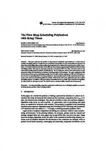
Figure 4 top shows the performance of the algorithms over different timeouts. For space constraints, we only show three representative cases. It is observed that each algorithm improves with larger timeouts. Overall, CGLS3 achieves better performance than other algorithms. While so far we presented summarised results over groups of instances, Figure 4 middle shows detailed results on each of the 120 instances when RSb-RCb and SDST125 scenario combination is used. Clearly CGLS3 significantly outperforms other algorithms. However, ARPDs of all solvers increases in the large problem instances, particularly when n ≥ 50. For space constraints, we do not show such instance-wise detailed results for other scenarios. Since there is no lower bound for the studied problem, we compare our results with some lower bounds of makespan obtained by using related problems. When optimal values are not known, lower (or upper) bounds are often obtained by relaxing some constraints and solving the relaxed problems. Assuming no blocking constraints, we can transform our proposed PFSP variant to the PFSP variant only with SDSTs. Then, making further assumption that SDSTs are all zero, we can obtain typical PFSPs. Given the 120 instances by (Taillard 1993), unfortunately, no optimal solution is known either for PFSPs or for PFSPs with SDSTs. Nevertheless, it is obvious that given a problem instance, optimal makespan for the typical PFSP version will be smaller than the optimal makespan for the PFSP variant with SDSTs, which will be smaller than the optimal makespan for the PFSP variant with SDSTs and mixed blocking constraints. In the absence of optimal values for the mentioned PFSP variants, we compare our results with the best known makespan values of the typical PFSPs (Tasgetiren et al. 2017b) and PFSPs with SDSTs (Ruiz and St¨utzle 2008). However, we note that these comparisons are just indicative and not definitive. Figure 4 bottom shows these results. Notice that the more the SDST periods the wider the gap between the best known makespans for typical PFSPs and that for PFSPs with SDSTs; which is expected. Interestingly, the more the SDST periods, the closer the gap between CGLS3 produced makespans for our proposed variant and the best known makespan for PFSPs with SDSTs. Overlapping of SDSTs and blocking times is behind this.

Figure 3: Comparison using 99% confidence interval.

Table 5: ARPD of algorithms for different scenarios. Blocking scenario

SDST scenario SDST10

SDST50 RSb-RCb SDST100

SDST125

SDST10

SDST50 RSb SDST100

SDST125

SDST10

SDST50 RCb SDST100

SDST125

τ 30 60 90 30 60 90 30 60 90 30 60 90 30 60 90 30 60 90 30 60 90 30 60 90 30 60 90 30 60 90 30 60 90 30 60 90

Algorithm IGA GRASP CGLS1 CGLS2 CGLS3 0.67 0.82 0.68 0.59 0.53 0.48 0.57 0.50 0.49 0.39 0.34 0.42 0.36 0.40 0.28 0.70 0.93 0.79 0.61 0.59 0.51 0.65 0.57 0.50 0.42 0.37 0.49 0.42 0.41 0.31 0.87 1.14 1.00 0.74 0.70 0.67 0.83 0.73 0.63 0.50 0.50 0.60 0.54 0.51 0.37 1.15 1.39 1.24 0.87 0.79 0.79 1.03 0.89 0.70 0.59 0.55 0.75 0.65 0.56 0.43 0.67 0.93 0.71 0.68 0.48 0.49 0.68 0.52 0.52 0.35 0.36 0.49 0.39 0.38 0.26 0.81 1.17 0.95 0.61 0.61 0.60 0.83 0.71 0.57 0.44 0.44 0.62 0.52 0.46 0.31 1.09 1.47 1.14 0.81 0.76 0.79 1.05 0.87 0.64 0.56 0.55 0.77 0.63 0.54 0.39 1.31 1.88 1.51 0.96 0.94 1.00 1.34 1.09 0.80 0.69 0.71 0.98 0.78 0.65 0.50 0.76 0.88 0.72 0.54 0.50 0.51 0.58 0.47 0.43 0.33 0.34 0.39 0.32 0.36 0.22 0.94 1.18 0.91 0.63 0.73 0.63 0.80 0.60 0.51 0.49 0.42 0.52 0.42 0.41 0.32 1.34 1.36 1.27 0.88 0.98 0.87 0.93 0.86 0.68 0.64 0.58 0.62 0.59 0.56 0.42 1.47 1.53 1.54 0.93 0.92 0.95 0.98 0.99 0.79 0.76 0.63 0.67 0.66 0.63 0.50

Related Work Although the realistic nature, SDST-PFSP have not yet been studied well. (Gupta and Darrow 1986) proposed heuristics for only two machine problems while (Ruiz, Maroto, and Alcaraz 2005) proposed genetic and memetic algorithms, and (Ruiz and St¨utzle 2008) developed an insertion-based iterated greedy search procedure using the well-known NEHbased algorithm (Nawaz, Enscore, and Ham 1983) in initialisation, insertion operator in local search, and a greedy strategy in perturbation. Recently, (Vanchipura, Sridharan, and Babu 2014) proposed a variable neighbourhood descent (VND) algorithm employing two different heuristics in initialisation while (Sioud and Gagn´e 2018) proposed an enhanced migrating bird optimization (MBO) algorithm. A comprehensive review of scheduling research with setup times has been provided by (Allahverdi 2015).

205

Figure 4: Top: Sample performance of the algorithms over different timeouts; Middle: ARPDs of 120 PFSP instances with SDST125 and RSb-RCb when τ = 90; Bottom: Comparison against lower bounds of makespan obtained from related problem.

Conclusions

For RSb-PFSP, a number of methods i.e. a differential evolution algorithm (Wang et al. 2010), a GRASP algorithm (Ribas and Companys 2015), and an iterated greedy algorithm (Tasgetiren et al. 2017a) have been presented. On the other hand, for RCb-PFSP, an integer linear programming (ILP) model (Martinez de La Piedra 2005), an electromagnetism like (EM) algorithm (Yuan and Sauer 2007), and a genetic algorithm (Sauvey and Sauer 2012) have been found. Recently, RSb-RCb-PFSP has attracted much attention. For example, a genetic algorithm (Trabelsi, Sauvey, and Sauer 2012), a bee colony algorithm (Khorramizadeh and Riahi 2015), and a scatter search algorithm (Riahi et al. 2017) have been presented. A very recent work by (Takano and Nagano 2017) proposed a Mixed Integer Linear Programming (MILP) model for PFSPs with SDSTs and only RSb constraints, and presented a branch-bound algorithm for small instances with at most 10 machines and at most 20 jobs. As we can see, flowshops with both overlapable SDSTs and mixed RSb-RCb blocking constraints (or even flowshop with both SDSTs and only RCb blocking) has not been studied yet, despite being a realistic problem. In this work, we provide the computational model and propose constraintguided local search (CGLS) algorithms that embed the nature of the constraints (SDST and blocking constraints) into the search. This is one of the most logical steps, given the proposed PFSP variant is NP Hard.

In this paper, we considered a permutation flowshop scheduling problem (PFSP) with two simultaneous and real constraints: sequence-dependent setup times (SDST) and RSb-RCb blocking constraints. To the best of our knowledge, this is the first attempt to model these two constraints, and we described a computational model for makespan minimisation of the problem. We further developed constraintguided local search algorithms. We conducted a detailed experiment with a total of 480 benchmark instances. The results show that the proposed algorithms significantly outperform adapted state-of-the-art methods for related problems. We expect to extend this approach to more complex constraints for a wide range of real world production lines.

Acknowledgements This research is supported by the Australian Research Council under Grant DP150101618.

References Allahverdi, A. 2015. The third comprehensive survey on scheduling problems with setup times/costs. European Journal of Operational Research 246(2):345–378. Baker, K. R. 1974. Introduction to sequencing and scheduling. John Wiley & Sons.

206

Dudek, R.; Smith, M.; and Panwalkar, S. 1974. Use of a case study in sequencing/scheduling research. Omega 2(2):253– 261. Glover, F. 1997. Tabu search and adaptive memory programmingadvances, applications and challenges. In Interfaces in computer science and operations research. Springer. 1–75. Gupta, J. N., and Darrow, W. P. 1986. The two-machine sequence dependent flowshop scheduling problem. European Journal of Operational Research 24(3):439–446. Khorramizadeh, M., and Riahi, V. 2015. A bee colony optimization approach for mixed blocking constraints flow shop scheduling problems. Mathematical Problems in Engineering 2015. Li, X.; Wang, Q.; and Wu, C. 2009. Efficient composite heuristics for total flowtime minimization in permutation flow shops. Omega 37(1):155–164. Martinez, S.; Dauz`ere-P´er`es, S.; Gueret, C.; Mati, Y.; and Sauer, N. 2006. Complexity of flowshop scheduling problems with a new blocking constraint. European Journal of Operational Research 169(3):855–864. Martinez de La Piedra, S. 2005. Ordonnancement de syst`emes de production avec contraintes de blocage. Ph.D. Dissertation, Nantes. Mladenovi´c, N., and Hansen, P. 1997. Variable neighborhood search. Computers & Operations Research 24(11):1097–1100. Nawaz, M.; Enscore, E. E.; and Ham, I. 1983. A heuristic algorithm for the m-machine, n-job flow-shop sequencing problem. Omega 11(1):91–95. Rajendran, C. 1993. Heuristic algorithm for scheduling in a flowshop to minimize total flowtime. International Journal of Production Economics 29(1):65–73. Resende, M. G., and Ribeiro, C. C. 2014. Grasp: Greedy randomized adaptive search procedures. In Search methodologies. Springer. 287–312. Riahi, V., and Kazemi, M. 2016. A new hybrid ant colony algorithm for scheduling of no-wait flowshop. Operational Research 16:1–20. Riahi, V.; Khorramizadeh, M.; Newton, M. H.; and Sattar, A. 2017. Scatter search for mixed blocking flowshop scheduling. Expert Systems with Applications 79:20–32. Ribas, I., and Companys, R. 2015. Efficient heuristic algorithms for the blocking flow shop scheduling problem with total flow time minimization. Computers & Industrial Engineering 87:30–39. Ribeiro, C. C.; Uchoa, E.; and Werneck, R. F. 2002. A hybrid grasp with perturbations for the steiner problem in graphs. INFORMS Journal on Computing 14(3):228–246. Ruiz, R., and St¨utzle, T. 2008. An iterated greedy heuristic for the sequence dependent setup times flowshop problem with makespan and weighted tardiness objectives. European Journal of Operational Research 187(3):1143–1159. Ruiz, R.; Maroto, C.; and Alcaraz, J. 2005. Solving the flowshop scheduling problem with sequence dependent setup

times using advanced metaheuristics. European Journal of Operational Research 165(1):34–54. Sauvey, C., and Sauer, N. 2012. A genetic algorithm with genes-association recognition for flowshop scheduling problems. J. of Intelligent Manufacturing 23(4):1167–1177. Sioud, A., and Gagn´e, C. 2018. Enhanced migrating birds optimization algorithm for the permutation flow shop problem with sequence dependent setup times. European Journal of Operational Research 264(1):66–73. Taillard, E. 1993. Benchmarks for basic scheduling problems. European Journal of Operational Research 64(2):278–285. Takano, M. I., and Nagano, M. S. 2017. A branch-andbound method to minimize the makespan in a permutation flow shop with blocking and setup times. Cogent Engineering 1389638. Tasgetiren, M. F.; Kizilay, D.; Pan, Q.-K.; and Suganthan, P. N. 2017a. Iterated greedy algorithms for the blocking flowshop scheduling problem with makespan criterion. Computers & Operations Research 77:111–126. Tasgetiren, M. F.; Pan, Q.-K.; Kizilay, D.; and V´elezGallego, M. C. 2017b. A variable block insertion heuristic for permutation flowshops with makespan criterion. In Evolutionary Computation (CEC), 2017 IEEE Congress on, 726–733. IEEE. Trabelsi, W.; Sauvey, C.; and Sauer, N. 2012. Heuristics and metaheuristics for mixed blocking constraints flowshop scheduling problems. Computers & Operations Research 39(11):2520–2527. Vanchipura, R.; Sridharan, R.; and Babu, A. S. 2014. Improvement of constructive heuristics using variable neighbourhood descent for scheduling a flow shop with sequence dependent setup time. Journal of Manufacturing Systems 33(1):65–75. Wang, L.; Pan, Q.-K.; Suganthan, P. N.; Wang, W.-H.; and Wang, Y.-M. 2010. A novel hybrid discrete differential evolution algorithm for blocking flow shop scheduling problems. Computers & Operations Research 37(3):509–520. Wang, L.; Pan, Q.-K.; and Tasgetiren, M. F. 2011. A hybrid harmony search algorithm for the blocking permutation flow shop scheduling problem. Computers & Industrial Engineering 61(1):76–83. Yuan, K., and Sauer. 2007. Application of EM algorithm to flowshop scheduling problems with a special blocking. In Proceedings of the ISEM.

207