mask result λ1 = 0.98 λ1 = 0.88 λ1 = 0.77 mask (t = 2) mask (t = 16) result (t = 16). Figure 1: Color editing ... aware selection masks in images containing textured regions with fuzzy and/or .... Anisotropic diffusion [Perona and Malik 1990; Black et al. 1998] is ..... The goal is to apply a warming filter to the city buildings and a.
Diffusion Maps for Edge-Aware Image Editing Zeev Farbman The Hebrew University
Raanan Fattal The Hebrew University
Dani Lischinski The Hebrew University
Abstract Edge-aware operations, such as edge-preserving smoothing and edge-aware interpolation, require assessing the degree of similarity between pairs of pixels, typically defined as a simple monotonic function of the Euclidean distance between pixel values in some feature space. In this work we introduce the idea of replacing these Euclidean distances with diffusion distances, which better account for the global distribution of pixels in their feature space. These distances are approximated using diffusion maps: a set of the dominant eigenvectors of a large affinity matrix, which may be computed efficiently by sampling a small number of matrix columns (the Nystr¨om method). We demonstrate the benefits of using diffusion distances in a variety of image editing contexts, and explore the use of diffusion maps as a tool for facilitating the creation of complex selection masks. Finally, we present a new analysis that establishes a connection between the spatial interaction range between two pixels, and the number of samples necessary for accurate Nystr¨om approximations. Keywords: diffusion maps, edge-preserving smoothing, edgeaware interpolation, edit propagation, Nystr¨om method
1
Introduction
Edge-aware operations, such as edge-preserving smoothing and edge-aware interpolation have recently emerged as useful tools for a variety of image editing and manipulation tasks: edge-preserving smoothing operators are widely used to extract and/or remove details from an image, e.g., [Chen et al. 2007; Farbman et al. 2008; Subr et al. 2009]; edge-aware interpolation makes it possible to propagate a set of sparse user-specified constraints (edits) in an intuitive manner by accounting for strong edges in the image, e.g., [Levin et al. 2004; Lischinski et al. 2006; Yatziv and Sapiro 2006; Li et al. 2008]. Most edge-aware interpolation approaches are based on local propagation of sparse user constraints. They use affinities between adjacent pixels to formulate and solve an optimization problem [Levin et al. 2004], or to perform blending using intrinsic (geodesic) distances [Yatziv and Sapiro 2006]. While such approaches provide the user with good local control, they have difficulty propagating sparse edits across strongly textured regions (Figure 1, top row), and can’t handle fragmented regions. Several solutions have been recently proposed to address these issues. In particular, the global all-pairs approach [An and Pellacini 2008] was demonstrated to be well-suited for propagating sparse (and possibly rough) user edits to large spatial neighborhoods. We discuss all these approaches in more detail in the next section. In this work we improve the performance of existing edge-aware
input + scribbles
mask
result
λ1 = 0.98
λ1 = 0.88
λ1 = 0.77
mask (t = 2)
mask (t = 16)
result (t = 16)
Figure 1: Color editing using local edit propagation. Top row: input, influence mask for the white scribble (using Lischinski et al. [2006]), and the corresponding result. Middle row: three leading eigenvectors of the diffusion map. Bottom row: masks produced using diffusion distances with different values of t, and final result. methods and extend them in several respects. We observe that some of the difficulties encountered by existing local propagation methods stem from the fact that the affinities they use are typically given by a simple monotonic function of the Euclidean distance between the low-level feature vectors associated with each pixel. This measure of similarity does not account for any higher level structure, which becomes apparent when one examines the distribution of pixel values in their feature space. We propose to address this shortcoming, and provide pairwise affinities with the missing global perspective, by leveraging the concept of diffusion distances, which has recently emerged in the spectral clustering literature [Coifman and Lafon 2006]. In natural images, where the number of distinct homogeneous regions is typically much smaller than the number of pixels, diffusion distances may be effectively approximated using a small number of diffusion maps: the eigenvectors of the pairwise affinities matrix (Figure 1, middle row). These maps, described in more detail in Section 3, also make it easy to compute diffusion distances corresponding to different times, providing an important parameter with which the user can control the desired amount of propagation (Figure 1, bottom row). In Section 4, we explore the benefits of using diffusion distances in a variety of edge-aware image editing contexts, and also demonstrate that diffusion maps facilitate the creation of complex edgeaware selection masks in images containing textured regions with fuzzy and/or fragmented appearance. Diffusion maps may be effectively approximated using a Nystr¨om method [Fowlkes et al. 2004]. This approach involves sampling a small number of columns of the (low rank) affinity matrix. A similar approximation was used by An and Pellacini [2008] in order to solve the associated dense linear system that arises in their all-pairs
approach. However, limiting the spatial range of permitted interactions between pixels raises the rank of the affinity matrix, and renders the approximation less accurate. In Section 5 we refine the analysis of An and Pellacini to obtain a more accurate estimate of the rank of the affinity matrix, as a function of the maximum distance in the image at which pixels are allowed to interact directly. The refined analysis enables one to determine the appropriate number of matrix columns to sample, in order to guarantee an accurate Nystr¨om approximation. Our analysis also shows that even with the increased sampling rates, the resulting matrices are sparse and thus can be solved efficiently using standard sparse linear solvers. This makes it possible to perform edge-aware image editing with an arbitrary permitted interaction range.
2
Previous Work
A number of techniques for edgeaware interpolation have been recently explored. Levin et al. [2004] introduced an optimization framework for colorizing grayscale images by propagation from a set of sparse user-provided constraints. This approach was generalized to other tonal manipulations [Lischinski et al. 2006], as well as to natural image matting [Levin et al. 2008a]. Yatziv and Sapiro [2006] propagate similar constraints by intrinsic (geodesic) distance based blending. All of the techniques above rely on gradients between adjacent pixels to control propagation, and thus have trouble propagating information in highly textured regions, as well as preventing propagation across low-contrast edges. Handling fragmented (disconnected) regions is another problem, since they might require many constraints to be provided by the user. Edge-aware interpolation.
An and Pellacini [2008] generalized optimization-based edit propagation to consider interactions between all pairs of pixels in the image, enabling less precise specification of user constraints and their propagation across disconnected regions. This approach results in a large dense affinity matrix, but this matrix is approximately low-rank, and can be approximated by sampling just a small number of columns (Nystr¨om method) [Williams and Seeger 2000]. Xu et al. [2009] have recently proposed to accelerate the all-pairs approach further by computing the propagation between pairs of clusters in feature space, rather than between pairs of pixels. An and Pellacini’s error analysis shows that the Nystr¨om approximation becomes less accurate as the spatial range of the interactions is decreased. However, since their goal is to enable edit propagation to rather large spatial neighborhood, they were able to achieve satisfactory results using a constant number of samples (100). In our work we also apply the Nystr¨om method to a related eigenvalue problem [Fowlkes et al. 2004], and present a refined error analysis that more precisely quantifies the effective rank of the affinity matrix as a function of the spatial interaction range, enabling us to generalize the all-pairs approach to handle arbitrary interaction ranges accurately and efficiently. ScribbleBoost [Li et al. 2008] is another approach that improves propagation across textured or fragmented regions. The user’s scribbles are used to perform supervised classification of the pixels, and the results are introduced into the optimization as additional soft constraints. A selection mask is then computed by solving the linear system once for each scribble type. While our idea of using diffusion distances also leverages machine learning techniques, we effectively perform unsupervised clustering, which considers all of the data in the image, rather than just the pixels covered by a particular set of strokes. Furthermore, the resulting diffusion distances are useful in such applications as edge-preserving smoothing, where no user input is available. Edge-preserving smoothing is used in a wide variety of computational photography applications [Farbman et al. 2008]. Popular edge-preserving smoothing filters Edge-preserving smoothing.
include the bilateral filter [Tomasi and Manduchi 1998], for which a number of efficient implementations have been proposed [Durand and Dorsey 2002; Paris and Durand 2006; Chen et al. 2007]. Fattal [2007] explored a fast iterative multiscale variant of the bilateral filter, while Farbman et al. [2008] advocated the use of weighted least squares optimization instead. Recently, Fattal [2009] introduced edge-avoiding wavelets, and demonstrated their usefulness for very fast edge-preserving smoothing, as well as for edge-aware editing. These techniques can also be applied to edit propagation, via interactive painting with edge-aware brushes [Chen et al. 2007], or by fast edge-aware pushing and pulling of the sparse constraints [Fattal 2009]. All of the techniques mentioned above rely on the difference between pixel values (difference in luminance, or Euclidean distance in some color space). Thus, we argue that they could all benefit from using diffusion distances instead, and support our claim by a number of examples in Section 4. Anisotropic diffusion [Perona and Malik 1990; Black et al. 1998] is another popular approach for edge-preserving smoothing via nonlinear PDE-based filtering. Although our work employes similar terminology (i.e., diffusion and time), our focus is on the unsupervised preconditioning of the data, independent of a particular smoothing or propagation scheme. Although not explored in this paper, one could conceivably use the resulting diffusion distances in the computation of the edge-stopping term of various anisotropic diffusion schemes. Subr et al. [2009] have recently proposed an edge-preserving smoothing approach based on identifying and fitting envelopes to local extrema in the image. This approach effectively assumes an oscillatory model of textured regions, and succeeds in removing detail even in high-contrast textured regions. While our approach does not make use of such a texture model, we show that by plugging diffusion distances into an existing edge-preserving smoothing approach it becomes possible to remove detail just as effectively. The scale of the details to be removed may be controlled via the time parameter, which is built into the diffusion distances that we use. Diffusion maps have emerged in the machine learning community as a tool for dimensionality reduction and unsupervised clustering [Coifman and Lafon 2006; Nadler et al. 2005; Singer et al. 2009]. This tool belongs to a larger family of spectral clustering techniques, which includes other closely related methods, such as locally-linear embeddings (LLE) [Roweis and Saul 2000], Isomaps [Tenenbaum et al. 2000], and Laplacian eigenmaps [Belkin and Niyogi 2003]. In particular, spectral clustering methods have been used to perform hard (binary) segmentation [Shi and Malik 1997; Weiss 1999] by thresholding the eigenvectors of suitably formed matrices. Meila and Shi [2001] pointed out the connection between these methods and Markov random walks. Diffusion distances also have a random walker interpretation (Section 3.1). However, in contrast to these methods, we are not interested in hard segmentation, but rather in deriving new distances to assist in edgeaware interpolation and smoothing. Clustering.
The use of random walks for segmentation was also explored by Grady [2006]. His formulation yields a linear system defined by an inhomogeneous Laplacian matrix, similar to the ones that arise in optimization-based edit propagation. Recently Grady suggested to accelerate his segmentation approach by precomputing a small number (40–80) of eigenvectors [Grady and Sinop 2008]. However, since his random walker formulation considers only limited spatial neighborhoods, our analysis in Section 5 implies that such an approximation is only accurate for small images. Spectral clustering has also been used for natural image matting [Levin et al. 2008b], where the eigenvectors of a suitable Laplacian matrix are rotated and combined together to yield a soft matte. We
also compute eigenvectors, but use them in order to define robust distances between pairs of image pixels. Another family of relevant works from the computer vision literature are path-based clustering methods, which examine the distribution of the data in some (typically high-dimensional) feature space, e.g., [Fischer and Buhmann 2003; Chang and Yeung 2008]. In particular, Omer and Werman [2006] measure the affinity between pixels in terms of the length and the density of the paths connecting them in color space. All of these methods, however, are very costly to compute. Diffusion distances also account for length and density of paths in the data, but lend themselves to faster computation. In addition, diffusion maps have a built-in notion of time, which makes it possible to control the granularity (scale) of the clusters in an efficient and intuitive manner.
3
Diffusion Maps
In this section we present our approach towards edge-aware image editing, which is based on the use of diffusion distances in place of the distances typically used by existing edge-aware methods. Existing edge-aware methods rely on a pairwise similarity (affinity) measure between image pixels. The affinities used in practice are typically a monotonic function of the distance between the pixels in some simple feature space, for example: k(xi , x j ) = exp(−kxi − x j k2 /2σr2 ),
(1)
where xi is the feature vector associated with the i-th pixel, e.g., its luminance or log-luminance, its coordinates in some color space, or a concatenation of color and spatial coordinates. Intuitively, the affinity between two pixels predicts the likelihood that both pixels belong to the same surface/region in the image. Edge-preserving smoothing techniques allow groups of pixels with high affinities between them to be averaged together, and edge-aware editing systems allow edits to propagate between pairs of pixels with high affinity. Thus, existing edge-aware methods are driven by the Euclidean distances between feature vectors corresponding to the pixels in the image. The shortcomings of this approach are that it might (i) fail to distinguish between regions separated by a low contrast edge; and (ii) fail to cluster together pixels in highly textured regions, which may exhibit strong differences between nearby pixels. While it is possible to discriminate between textures by augmenting the feature vectors with texture descriptors such as responses to Gabor filter banks [Turner 1986] or histograms of such responses [Malik et al. 2001], these descriptors aggregate information from a fairly large window around each pixel, and thus effectively operate at a lower spatial resolution. We argue that pairwise distances among the data points provide only partial (and sometimes misleading) information about the manner in which pixels should be clustered. Additional highly relevant information may be obtained by examining the actual distribution of the data in the feature space. Consider, for example, the image shown in Figure 2. The distribution of the pixel colors in this image is highly non-uniform, and clearly exhibits three distinct clusters corresponding to the blue sky region, the red flowers, and the green grass. While the pairwise distances in the color space between the red and the green pixels are of the same order of magnitude as those between red and blue (or green and blue), the distribution reveals that the transition between the red and the green clusters is much more densely populated than the red-blue or green-blue transitions. This corresponds to our intuition that in the coarsest possible clustering of this image the green and red should go into one cluster, while the blue into another. Thus, we would like pixel affinities to account for the actual distribution of the data in the feature space. Intuitively, the likelihood of
two data points to belong to the same cluster should depend on the lengths and the density of the different paths between them. This may be achieved by replacing the Euclidean distances with diffusion distances, a concept that was recently proposed for dimensionality reduction and clustering [Coifman and Lafon 2006; Nadler et al. 2005], which we describe in more detail below.
3.1
Diffusion distances and diffusion maps
Definitions. Given a set of n data points, x1 , . . . , xn in some feature space, we define a pairwise affinity matrix W , where Wi, j = k(xi , x j )
(2)
for some affinity function k(·, ·). Let D be a diagonal normalization matrix Di,i = ∑ j Wi, j . The normalized matrix M = D−1W can be interpreted as a stochastic matrix, where Mi, j is the probability of a random walker located at point xi to transition to point x j in a single time step. Consequently, Mt consists of the probabilities to move from each point to another in t time steps. Informally, for each t, we can associate Mt with a “soft” clustering of the data points: a subset of points is considered a cluster if there is a low probability of a random walker starting from a points in this subset to end up outside it after t moves. In general, these clusters tend to become coarser as t increases. Diffusion distance. There is an interesting relationship between the geometry of the data and the spectral properties of M, captured by the notion of diffusion distances [Nadler et al. 2005]. The diffusion distance Dt (xi , x j ) is defined as difference between the probabilities that a random walker starting at each of these two points will end up in the same position at time t. Formally, Dt2 (x, y) = ∑ (p(t, z|x) − p(t, z|y))2 w(z),
(3)
z
where p(t, z|x) is the probability of a random walker to transition from x to z in t time steps, and w(z) is the reciprocal of the local density at z. Intuitively, the more short paths connect two points, the smaller the diffusion distance between them. Note that (3) defines a family of diffusion distances parameterized by the time t. As t increases, two points that were originally distant from each other may grow closer. Diffusion map. It may be shown that M has a set of n real eigenvalues {λi }n−1 0 . Furthermore, if all the points are connected (i.e., there is a path of non-zero probability between any two points), then M has a unique eigenvalue equal to 1, and the other eigenvalues form a non-increasing sequence of non-negative numbers: λ0 = 1 > λ1 ≥ λ2 ≥ · · · ≥ λn−1 ≥ 0. Denoting by ψ0 , . . . , ψn−1 the corresponding right eigenvectors of M, the diffusion map at time t is defined as a mapping between the original data points and the eigenvectors (each scaled by its corresponding eigenvalue): � t ψn−1 (x) . (4) Ψt (x) = λ1t ψ1 (x), λ2t ψ2 (x), . . . , λn−1 Note that the eigenvector ψ0 does not participate in the diffusion map, since it is constant and thus does not contribute any discriminating information. As shown by Nadler et al. [2005], the diffusion distances at time t may be expressed simply as Euclidean distances in the corresponding diffusion map: Dt (x, y) = kΨt (x) − Ψt (y)k2 .
(5)
In other words, the diffusion distance between two points is simply the sum of squared differences between the corresponding entries of the eigenvectors ψi , where each eigenvector is weighted by λit . In practice, the matrix M often exhibits a spectral gap, i.e., only a few of its eigenvalues are close to one, while the rest are much
ψ1 , λ1 = 0.998
t = 256
ψ2 , λ2 = 0.968
t = 64
ψ3 , λ3 = 0.908
t = 16
example image
40
20
b
0
−20
−40
−60
60
50
40
30
20
10
0
a
−10
−20
60 80 20 40 L
pixels in LAB space
Figure 2: Left: highly non-uniform distribution of pixel colors in an image. Middle: the three leading eigenvectors of the normalized pairwise affinity matrix reveal the dominant clusters. Right: gradients computed using diffusion distances at different times. smaller. Thus, the diffusion distance is well approximated by a diffusion map constructed from the first k eigenvectors, with the accuracy of the approximation increasing with the time t. As discussed in Section 5, the value of k depends on the spatial support of the affinity kernel. Example. Figure 2 shows a visualization of the first three eigenvectors produced from the input image. Note that the first eigenvector ψ1 roughly clusters the image into two main regions (corresponding to sky and ground), ψ2 mainly distinguishes the red flowers from everything else, while ψ3 sets apart the white clouds from everything else. The next eigenvectors (not shown), corresponding to smaller eigenvalues further separate between progressively smaller regions in the image. Since all eigenvalues are strictly smaller than 1, increasing the value of the time parameter t gives more weight to the “coarser” eigenvectors. Thus, diffusion distances corresponding to higher values of t emphasize edges separating between the coarser clusters, while suppressing those that separate smaller scale image regions. In the Section 4 we demonstrate the usefulness of diffusion distances by plugging them in place of regular pairwise distances in several edge-aware operations.
3.2
Efficient implementation
A possible concern regarding the use of diffusion distances in practice is the added computational cost. Specifically, a naive implementation would involve forming the all-pairs normalized affinity matrix M = D−1W and then computing the leading eigenvalues and eigenvectors of this matrix in order to form the diffusion maps. This is impractical for working with high-resolution images. In order to make the approach practical we use the approximation proposed by Fowlkes et al. [2004], which is based on the Nystr¨om method. The Nystr¨om approximation method proceeds as follows. Given
an image with N pixels, distribute a small number m of samples across the image. Next, compute two matrices: an m × m matrix A, which consists of the pairwise affinities among the m samples, and an (N −m)×m matrix B, of the affinities between these samples and the rest of the image. This corresponds to partitioning the complete N × N affinity matrix W as: � � A BT W= (6) B C Note that the block C, which contains the bulk of the pairwise affinities is never actually computed. The approximate eigenvectors Ve of W are then given as � � V e V= , (7) B V Λ−1 where V are the eigenvectors of A, and Λ is the corresponding diagonal eigenvalue matrix. Intuitively, we compute the eigenvalues and eigenvectors of the sampled matrix A, and use B to “upsample” these vectors to the full resolution of the original problem. This approximation yields the eigenvectors of W , while the diffusion map consists of the eigenvectors of M = D−1W , where Di,i = ∑ j Wi j . Fowlkes et al. [2004] show how to approximate these row sums using only A and B, and we refer the reader to their article for further details, and the pseudocode of the complete procedure. Thus, a practical method for computing the diffusion maps involves sampling the image. In Section 5 we show that, for a given accuracy, the number of samples depends on N/τ 2 , where τ is the pairwise interaction range between pixels. Therefore, if the affinity matrix allows all pairs of pixels to interact, a constant number of samples will suffice. The exact number depends on the image at hand, since the reduced matrix should ideally represent the main
Figure 3: Local edit propagation. Top: input with scribbles and result using ordinary distances (middle) and diffusion distances (right), computed with spatial coordinates (t = 16). Bottom: The corresponding influence maps for the green scribble.
Figure 4: WLS edge-preserving smoothing. Top: input and smoothing (λ = 10) using color gradients (middle) and diffusion distances (left, t = 4). Bottom: results after local contrast adjustments.
distinct regions present in the image. The samples are placed using stratified sampling of the image, as was also done by An and Pellacini [2008]. The following times (in seconds) were measured1 when constructing a diffusion map with 7 eigenvectors for different image sizes and numbers of samples: 10 samples 30 samples 60 samples
4
0.5 MP 0.58 1.24 2.44
0.75 MP 0.58 1.82 3.66
1 MP 0.79 2.46 4.95
1.5 MP 1.12 3.57 7.20
2 MP 1.53 4.84 9.75
Experimental Validation
In order to evaluate the practical benefits of using diffusion distances in place of regular pairwise distances between the original data points, we experimented with a variety of common edge-aware operators. For each operator we compare its performance with and without the use of diffusion distances. Note that it is not our intention to demonstrate that one is able to achieve perfect results simply by switching to diffusion distances, nor do we claim that similar results could not have been achieved in any other way. Rather, we aim to show that there are practical scenarios where state-of-theart methods perform better with diffusion distances, given the same input. We experimented with a number of color spaces when computing the affinity matrices, and for all the results shown in this paper we use the CIELAB color space (normalized such that the L channel range is [0, 1]). The affinities are defined by the Gaussian kernel (1) with σr2 = 0.1 for edge-preserving interpolation and smoothing, and σr2 = 0.25 for matting. We have also experimented with a number of different feature vectors. Using the pixel colors along with spatial coordinates is an attractive option, since it typically yields good results. However, it reduces the spatial interaction range between pixels, and therefore requires using more Nystr¨om samples to compute the diffusion map, as shown in Section 5. For that reason, in all of our results except Figures 3 and 9, we use only the color at each pixel (no spatial attenuation), and compute diffusion maps using 30 samples. Our attempts to enrich the feature vectors with simple texture descriptors (such as Gabor filter banks), were not successful so far and this is left as a possible direction for a future work. Throughout this section, for each result using the diffusion distances we report the value of t which we used. Possible strategies for setting this parameter are discussed in Section 6. 1 Using
C++ and Matlab on a 2.8 GHz Intel Core 2 Duo processor.
input image
[Subr et al. 2009]
WLS with diffusion
Figure 5: A comparison with the method of Subr et al. [2009]. Local edit propagation. Figure 1 demonstrates the performance of diffusion distances in the context of local edit propagation from sparse user constraints by plugging these distances into the optimization-based approach described by Lischinski et al. [2006]. The goal is to apply a warming filter to the city buildings and a cooling filter in the sky and water regions using minimal user input. This is a challenging task, due to the many very high-contrast transitions between the buildings. Indeed, the original method fails to propagate the yellow scribble to capture the entire region of interest. When using diffusion distances with t = 2 the result is slightly better, but increasing the time to t = 16 nicely captures the target area, and produces a significantly better result.
In Figure 3 the goal is to change the hues of two adjacent strongly textured regions. Although the two regions appear quite distinct to a human observer, selecting each of them using state-of-the-art commercial tools proved to require a substantial amount of user interaction. Using again the method of Lischinski et al. [2006] we were not able to obtain a satisfactory result with a sparse set of scribbles, since the gradients between the two regions and inside each region are of the same order of magnitude. Switching to diffusion maps constructed using the color at each pixel only produced a similar unsatisfactory result. However, by adding the spatial coordinates to the feature vectors and feeding the resulting diffusion distances into the same method, we were able to produce a more satisfactory result. The supplementary material contains additional local editing results, as well as examples of using diffusion distance in the context of the distance-based blending approach of Yatziv and Sapiro [2006]. Similar improvements in propagation may be observed there as well. In practice, scribble-based editing is intended for an iterative interactive workflow, where the user is able to add or remove scribbles until a satisfactory result is achieved. With sufficient amount of user input it is obviously possible to achieve results that are identical or better than those that we have shown. Thus, the practical advantage of using diffusion distances in this context lies in reducing the amount of necessary user input.
user. However, in complex fragmented regions one might want to apply a different adjustment to different parts of the region. For example, in Figure 7, modifying the color of the soil and the bushes independently is difficult to accomplish using scribble-based local propagation. An experienced Photoshop user might prefer first to create a mask separating the ground from the sky, and then use color range selection tools to further separate the ground to reds and greens. Here we demonstrate that having diffusion maps under the hood can also be useful for quickly obtaining similar fuzzy masks.
Figure 6: Closed form matting with diffusion distances. Top: input and ground truth. Bottom: corresponding results without (left) and with diffusion distances (right, t = 2). Figure 4 compares the results of filtering an image with the WLS edge-preserving smoothing operator [Farbman et al. 2008] with and without the use of diffusion distances. This example contains textures with high gradients on the buildings in the background. The WLS operator controls the degree of smoothing via a parameter λ . When the value of λ is chosen so as to remove most of the texture form the building, this results in faded edges between the buildings and the sky (top middle image). Such contrast reduction is undesirable for applications such as image abstraction. When the same operator uses diffusion distances, the contrast of these edges is better preserved (top right). The bottom row shows what happens when the removed texture detail is amplified and added back in (local contrast boost). It may be seen that the detail on the buildings is boosted in a much more uniform manner on the right.
Edge-preserving smoothing.
Figure 5 shows a comparison between a result produced by the method recently proposed by Subr et al. [2009], and the result of edge-preserving filtering with WLS using diffusion distances. Subr et al. first search for the local extrema in the image, and then fit a lower and an upper envelope to these extrema by solving a linear system twice. It may be seen that WLS with diffusion distances is able to remove the small scale detail on the vase just as effectively, while avoiding the costs of non-linear filtering or solving multiple linear systems. Both methods are still unable to smooth out coarser texture and leave room for future work. We also experimented with incorporating the diffusion distance into matting method by Levin et al. [2008a]. Unlike many matting algorithms that assume a tight trimap, this method also admits sparse user scribbles indicating background and foreground, which are propagated over the image to yield an alpha matte. We have modified the authors’ original code to use diffusion coordinates instead of colors when constructing the matting Laplacian. Figure 6 shows an example where the modified method produces a matte that is closer to the ground truth than the original method. As with local image editing, we found that fewer scribbles are necessary to produce an accurate matte with diffusion distances in the presence of textured regions. To further evaluate the matting performance, we also ran the benchmark suggested in [Rhemann et al. 2009], but we did not see any significant increase in quantitative accuracy. This can be explained by the fact that this benchmark uses tight trimaps; thus, the ability of diffusion distances to propagate across textured regions does not play a significant role. When the input trimap is loose, the visual accuracy of the diffusion-based mattes is sometimes better (see the supplementary materials). Matting.
4.1
Fuzzy Selection with Diffusion Maps
In local edit propagation, a particular adjustment is propagated and applied to all the pixels within a contiguous region indicated by the
Recall that diffusion maps consist of the dominant eigenvectors of the all-pairs affinity matrix, which discriminate between the dominant modes in the data at various scales. Each eigenvector consists of positive and negative values (shown in shades of red and blue in Figures 1 and 2), with the transitions between negative and positive regions corresponding to transitions between clusters. Thus, our idea is that given a scribble drawn by the user we first identify which of the eigenvectors in the diffusion map “responds” most strongly to this scribble by measuring the variance of each eigenvector in the pixels covered by the scribble. Having found such an eigenvector we use it to produce a mask that captures either the positive or the negative regions of this eigenvector. Formally, given a user scribble S we first search for the eigenvector ψi which exhibits the highest variance in the area covered by the scribble: arg max Var {λi ψi (x)}x∈S . (8) i
We then use this eigenvector to define two masks, for the areas where the eigenvector is positive and negative, respectively: Mψ+i =
exp(ψi )a exp(ψi )a + exp(−ψi )a
and Mψ−i = 1 − Mψ+i
(9)
where the parameter a enables the user to control the hardness of the masks (a < 1 makes the masks softer, while a > 1 makes them harder). Note that the masks are normalized such that their sum at every pixel is 1. It is often the case that the first eigenvector ψ1 effectively partitions the image into two main regions (e.g., ground and sky, as seen in Figures 1 and 2). Thus, if the scribble S is contained in one of these two regions, we assume that it is the user’s intent to apply the manipulation only inside the containing region. In this case, we also define an attenuation mask: ( + Mψ1 ∑x∈S ψ(x) > 0 Matt = (10) Mψ−1 ∑x∈S ψ(x) < 0 The final mask used to edit the image is then given by the product of one of the masks Mψ+i or Mψ+i with the attenuation mask Matt . The process is demonstrated in Figure 7. The user first draws a scribble across the boundary between the two main regions in the image (sky and ground). The first eigenvector responds most strongly to this scribble, yielding a mask distinguishing between the two regions, and the user is able to boost the local contrasts in the sky without significant effect elsewhere. The next scribble is drawn across the ground region, and the eigenvector that responds most strongly discriminates between the red soil and the green vegetation. The user uses one of the two resulting masks (Mψ+2 in this case) to change the hue and saturation of the soil, and its complement (Mψ+2 ) to make the vegetation more green, using a different hue/saturation adjustment. Here, attenuating by the mask of the first eigenvector helps confine the edit to the ground region (the figure shows the attenuated mask Matt Mψ+2 ). Finally, a scribble across the sky produces a mask that discriminates between the blue sky and the white clouds, enabling the user to deepen the color of the sky. Again, the edits are attenuated to apply only in the sky region, yielding the final result.
input image
mask 1
result 1
mask 2
result 2
mask 3
result 3
Figure 7: Red Canyon State Park, Utah. Each scribble produces a corresponding mask by selecting from the diffusion map the eigenvector with the highest variance under the scribble. The 2nd and 3rd masks are attenuated by the first eigenvector.
5
Analysis
The optimization-based edit propagation operators explored so far in the literature may be grouped into two main classes, based on the spatial range of the interactions that they explicitly account for. One class corresponds to short-range/local interactions, while the other to long-range/global (all-pairs) interactions. Below, we review the methods used for solving the edit propagation problem in each of these two cases, and conclude that these methods are not well suited for handling middle-range interactions. However, a careful spectral analysis of the corresponding affinity matrices leads naturally to a hybrid solution method that makes it possible to handle this intermediate case, both accurately and efficiently. Interaction range. Optimization-based edge-aware edit propagation methods solve a linear system of the form Lx = b, where L = D −W is a non-homogeneous Laplacian matrix, W is an affinity matrix, such as the one defined in eq. (2), and D is a diagonal matrix given by Di,i = ∑ j Wi, j . Let us define the spatial interaction range τ as the radius (in pixels) beyond which the pairwise affinity between two pixels in the image falls below some threshold ε. For example, the 5-point inhomogeneous Laplacian operator used in [Lischinski et al. 2006; Farbman et al. 2008] corresponds to τ = 1. Levin et al. [2004; 2008a] use a slightly larger (but still constant) interaction range, while the all-pairs approach [An and Pellacini 2008] uses an interaction range τ = O(n), where n is the dimension (width or height) of the image. The interaction range τ determines the manner in which sparse edits may propagate across the image. When τ is a small constant, edits propagate well within smooth contiguous image regions, but the propagation is blocked by strong edges in the image, so fragmented or strongly textured regions cannot be handled. At the other extreme, when τ = O(n), edits are allowed to propagate between regions of similar attributes, even if these regions are distant and completely separated by regions with very different color attributes. If one is interested in being able to handle fragmented regions, while at the same time having the flexibility of local control, using an intermediate interaction range 1 � τ � n might provide the answer. However, as we shall see below, in the latter case it is not clear how the resulting systems of linear equations can be efficiently computed and solved in practice. Existing approaches. Let us review the solution methods that are commonly used to handle the two extreme cases. The case of sparse Laplacian matrices has been studied extensively in the numerical computing literature, since such matrices are used for approximating differential operators. It is well known [Trottenberg et al. 2001] that such matrices have a condition number that grows as a function of n2 , and their eigenvectors correspond to modes with variations at different scales (Fourier modes at different wavelengths). There-
fore, such matrices are treated with multi-scale preconditioners that capture and rescale these modes, such as the geometric Multigrid method [Trottenberg et al. 2001], or conjugate gradient with hierarchical basis preconditioning [Szeliski 1990]. Non-homogeneous sparse matrices can be solved using operatordependent Multigrid, Algebraic Multigrid [Trottenberg et al. 2001] in O(N) time, where N is the dimension of the matrix (N = n2 ), or using the locally-adapted hierarchical basis preconditioner of Szeliski [2006]. Recently, several works showed that the actions performed by these non-homogeneous Laplacian systems can be approximated efficiently without explicitly constructing, preconditioning, and solving the full-resolution linear system [Kopf et al. 2007; Fattal 2009]. In contrast, the global all-pairs Laplacians behave differently: they are dense and hence linear relaxations such as Gauss-Seidel or conjugate gradient become prohibitively expensive, since each matrixvector multiplication costs O(N 2 ). In natural images, which typically consist of a limited number of regions, each containing a large number of pixels with similar attributes, the affinity matrix W is close to low rank. An and Pellacini [2008] exploit this observation, and use the Nystr¨om method [Williams and Seeger 2000], to first drastically reduce the dimensionality of the matrix and then solve the associated Laplacian in its reduced form, using the Woodbury formula [Golub and Van Loan 1998]. The total cost of this approach is O(m2 N), where m is the (small) number of samples. To summarize the discussion so far, a variety of efficient and accurate solutions exist for the two extreme cases of either very sparse or fully dense inhomogeneous Laplacians. These solutions are practically linear in the number of pixels N. However, these solutions are not well suited for the intermediate case of 1 � τ � n, since the corresponding affinity matrices are neither sufficiently sparse, nor sufficiently rank-deficient [An and Pellacini 2008]. Rank vs. interaction range. In order to propose an effective solution for these intermediate cases, let us first examine the manner in which the rank of the affinity matrix W depends on τ. The top right plot in Figure 8 shows several spectra of normalized Gaussian affinity matrices corresponding to increasing values of σs (and hence increasing values of τ). Note that for short interaction ranges, most eigenvalues are non-negligible, but their number indeed decreases as σs becomes larger. Plotting the numerical rank as a function of N/τ 2 (Figure 8, bottom left) reveals that as τ gets smaller, the rank grows approximately as N/τ 2 . In the spatially-homogeneous case (a constant, or very smooth image), this empirical result can be verified formally by noticing that W is a circulant matrix that corresponds to convolution with the affinity kernel, e.g., exp(−krk2 /σs2 ). In this case, the eigenvalues
1
m = 1.00
Therefore, we suggest the following strategy: start with some constant number (tens to a few hundred) samples for the all-pairs case, and increase the number of samples proportionally to N/τ 2 . This strategy is demonstrated in the bottom right plot of Figure 8, which confirms that the error corresponding to a constant number of samples increases as τ decreases, while using N/τ 2 samples results in a non-increasing error.
s
ms = 1.41 ms = 2.00 ms = 4.00 ms = 11.31
0.5
0 0 0.8
9000
5000
10000
15000
using 100 samples using N/o2 samples
0.6
Rank
Error
6000 0.4
3000 0.2
0 0
3000
N/o2
6000
9000
0
100
80
60 40 Spatial range (o)
20
Figure 8: Top left: an image from which several test windows with different amounts of detail were chosen. Top right: eigenvalues of affinity matrices for one of these regions. Bottom left: the effective rank as a function of N/τ 2 averaged over 70 randomly chosen 96 × 96 test windows (in blue). The red line starts at a constant value on the left and grows to full rank linearly in N/τ 2 , indicating our proposed sampling strategy. Bottom right: Nystr¨om approximation error as a function of τ for different sampling strategies, measured for one of the windows.
Edit propagation example. Figure 9 demonstrates the importance of using an appropriate sampling rate for edit propagation in practice. Suppose that given the input image the user wishes to recolor all of the tulips and marks a single tulip with one scribble, while placing another scribble across the background. The all-pairs approach is well-suited for this scenario, and the desired interaction range here is roughly the entire image. According to our analysis, a small constant number of samples suffices for this case. Indeed, the propagation masks obtained using a small (50) and a larger (500) number of samples look virtually identical, and produce the same visual result. In contrast, suppose the goal is to recolor only the left and right flowers, while keeping the original color in the middle. To achieve this goal with the all-pairs approach, the interaction range must be significantly reduced. In this case, using a small number of samples no longer produces the desired mask, which is nevertheless obtained with a suitably larger number of samples.
λk of W are given (up to scale) by [Oppenheim and Schafer 1975]
Efficient numerical solution. The analysis we have presented in this section, suggests not only the correct sampling rate to use with intermediate interaction ranges, but also how to efficiently solve the associated linear system D −W . According to the Nystr¨om approximation, � � A W ≈ UA−1U T , where U = B , (15)
λk ∝ exp(−σs2 kkk2 (2π/n)2 ),
(11)
and applying the Woodbury identity [Golub and Van Loan 1998] yields:
where k are the indices in the Fourier domain. Thus, the number of eigenvalues of W above some fixed threshold η is proportional to the number of different k’s that satisfy:
(D −UA−1U T )−1 = D−1 − D−1U(−A +U T D−1U)−1 D−1 . (16)
exp(−σs2 kkk2 (2π/n)2 )
>
η,
−σs2 kkk2 (2π/n)2
>
log(η),
kkk2