Feb 4, 2005 - the light like Wilson loops and show that it is equivalent to the ..... The generalized vacuum averaged Wilson loop operator W(CT ) is given by.
UPRF–92–354 hep-ph/9210281 September, 1992
arXiv:hep-ph/9210281v2 4 Feb 2005
Partonic distributions for large x and renormalization of Wilson loop ∗ G. P. Korchemsky†
‡
and G. Marchesini
Dipartimento di Fisica, Universit`a di Parma and INFN, Gruppo Collegato di Parma, I–43100 Parma, Italy
Abstract We discuss the relation between partonic distributions near the phase space boundary and Wilson loop expectation values calculated along paths partially lying on the lightcone. Due to additional light-cone singularities, multiplicative renormalizability for these expectation values is lost. Nevertheless we establish the renormalization group equation for the light like Wilson loops and show that it is equivalent to the evolution equation for the physical distributions. By performing a two-loop calculation we verify these properties and show that the universal form of the splitting function for large x originates from the cusp anomalous dimension of Wilson loops.
∗
Research supported in part by Ministero dell’Universt`a e della Ricerca Scientifica e Tecnologica. On leave from the Laboratory of Theoretical Physics, JINR, Dubna, Russia ‡ INFN Fellow
†
1.
Introduction
It is well known [1] that for hard distributions such as deep inelastic structure functions, fragmentation functions, Drell-Yan pair cross section, jet production etc. near the phase space boundary the perturbative expansion involves large corrections which needed to be summed [2, 3]. This region is characterized by the presence of two large scales Q2 and M 2 with Q2 ≫ M 2 ≫ Λ2QCD and at any order in perturbation theory the leading contributions are given by double logarithmic terms (αsn ln2n Q2 /M 2 ). The leading contributions can be summed and the result is given by the exponentiation of the one-loop contribution [4]. This exponentiated form holds also after the summation of the next-to-leading contributions (αsn ln2n−1 Q2 /M 2 ). The exponent is simply modified by two-loop corrections in which the term αs2 ln4 Q2 /M 2 is absent and the coefficient of αs2 ln3 Q2 /M 2 is proportional to the one-loop beta-function [5]. This fact suggests us to apply renormalization group approach for summing large perturbative contributions to all orders. The universal properties of hard processes near the phase space boundary originate from the universality of soft emission, which is responsible of the double logarithmic contributions. Soft gluon emission from fast quark line can be treated by eikonal approximation for both incoming and outgoing quarks. In the eikonal approximation quarks behave as classical charged particles and their interaction with soft gluons can be described by path ordered Wilson lines along their classical trajectories [6, 7]. The corresponding hard distribution is then given by the vacuum averaged product of the time-ordered Wilson line, corresponding to the amplitude, and the antitime ordered Wilson line, corresponding to the complex conjugate amplitude. The combination of these Wilson lines forms a path ordered exponential W (C) along a closed path C which lies partially on the light-cone and depends on the kinematic of the hard process � I � µ W (C) ≡ h0|P exp ig dzµ A (z) |0i , Aµ (z) = Aaµ (z)λa (1.1) C
where λa are the gauge group generator. Here the gluon operators are ordered along the integration path C and not according to time. Notice that on different parts of the path C the gluon fields are time or anti-time ordered. This expression is different from the usual Wilson loop expectation value in which one has ordering along the path for the colour indices of λa and ordering in time for the gluons fields Aaµ (z). In eq. (1.1) we have ordering both of colour matrices and gauge fields along the path. In this paper we study the renormalization properties of W (C) for a path C partially lying on the light-cone and show that renormalization group (RG) equation for W (C) corresponds to the evolution equation [8] for the parton distribution function or the fragmentation function near the phase space boundary. In particular, we discuss the relation between the “cusp anomalous dimension” of Wilson loop and the splitting function P (z) for z → 1. In sect. 2 we establish the relation between W (C) and the distribution function or fragmentation function near the phase space boundary. In sect. 3 we perform the two-loop calculation in the Feynman gauge and in the MS−regularization scheme of W (C) with the path C fixed by the kinematics of hard process. In sect. 4 we deduce the RG equation for W (C) and show in sect. 5 that this equation gives rise to the evolution equation for the distribution function and fragmentation function near the phase space boundary. Sect. 6 contains some concluding remarks.
2
2.
Wilson loop and structure function in the soft limit
Consider the deep inelastic process for an incoming hadron of energy E, longitudinal momentum Pℓ and mass M probed by a hard photon with momentum q. In the infinite momentum frame we have P+ ≫ P− , where the light-cone variables for the hadron momentum Pµ = (P+ , PT , P− ) are defined by √ √ P− = (E − Pℓ )/ 2, PT = (P1 , P2 ) = 0 . P+ = (E + Pℓ )/ 2, In this frame xP+ is the “+” component of the momentum of the quark probed by the hard photon, where x = −q 2 /2(P · q) is the Bjorken variable. For x → 1 the hard photon probes at short distances the quark which carries nearly all hadron momentum. In this region the hard process is characterized by two scales: the virtuality of the photon Q2 = −q 2 , which gives the short distance scale, and the large distance scale (1 − x)Q2 . In this Section we show that, after factorization of leading twist contributions, the partonic distributions for x → 1 are given in terms of a generalized Wilson loop in (1.1). To show this we first make the leading twist approximation and then we perform the x → 1 limit.
2.1.
Summing collinear gluons
Due to the factorization theorem [9] the differential cross-section of this process is given in terms of the partonic distribution function and the partonic cross section. The partonic distribution function is a universal distribution measuring the probability to find in the hadron a parton with x fraction of the P+ momentum. To leading twist (Q2 ≫ M 2 ) the quark distribution function has the following representation [10] � Z y � Z +∞ dy− −iP+ y− x µ ¯ e hP | Ψ(y) P exp ig dzµ A (z) γ+ Ψ(0) |P i , (2.1) F (x, µ/M) = 0 −∞ 2π where the vector yµ lies on the light-cone with components yµ = (y+ , yT , y− ) = (0, 0, y− ) . The state |P i describes the hadron with momentum P and mass M. Integration over y− fixes the value of the “+” component of the total momentum of the emitted radiation to be (1 − x)P+ . The corresponding transverse and “−” components are integrated over by fixing yT = 0 and y+ = 0. Because of these unrestricted integrations the structure function contains ultraviolet ¯ (UV) divergences which are subtracted at the reference point µ. The quark field operators Ψ(y) and Ψ(0) are defined in the Heisenberg representation. The path ordered exponential is evaluated along the line between points 0 and yµ on the light-cone and ensures the gauge invariance of the nonlocal composite quark–antiquark operator. In what follows we will intensively use properties of Wilson lines which will appear in our analysis. We now briefly describe the physical meaning of Wilson line entering into the definition (2.1). Let us start considering the general form of the structure function of the deep inelastic scattering as matrix element of two electromagnetic currents: Z d4 z −iqz e hP |j+ (z)j+ (0)|P i , (2.2) (2π)4 3
q
p′
k
p
Figure 1: One-loop Feynman diagram contributing to the structure function of deep inelastic scattering. The gluon with momentum k is emitted by the quark p and absorbed by the quark p′ in the final state. We use solid line for quarks, curly lines for gluons, wavy lines for photons and dot-dashed line for the unitary cut. where
¯ jµ (z) = Ψ(z)γ µ Ψ(z) .
It is well known that in the leading twist approximation the structure function is defined by contributions of Feynman diagrams in which only one of the quarks of the hadron |P i participates in the hard scattering § . One of these diagrams is shown in fig. 1. In the infinite momentum frame, in the leading twist limit one can neglect the transverse motion of the quark inside the hadron and put the velocity of quark equal to the hadron velocity, vµ = Pµ /M .
(2.3)
As we will show in sect. 3, all singularities of the distribution function for x → 1 are absorbed by Wilson loop depending on the quark velocity v rather than momentum. Consider for example the one-loop contribution of fig. 1 to (2.2). In the infinite momentum frame the incoming quark has momentum pµ with p− ≪ p+ whereas the recoiling momentum P ′ has component p′− ≫ p′+ . The vertices for the absorption and emission of the real gluon k are given by /pγµ (/p − k/) p/′ γµ (p/′ + k/) and −2pk + i0 2p′ k − i0 respectively. For vanishing quark mass the two vertices contain the following singularities: • p−collinear: k+ ∼ p+ ,
k − ∼ p−
• p′ −collinear: k+ ∼ p′+ ,
k− ∼ p′−
• soft:
k− ∼ k+ → 0 ,
with k2T = 2k+ k− . According to the LNK theorem [11], by summing all diagrams for the structure function both the p′ −collinear and the soft (or infrared) singularities cancel. We then focus our attention only on the p−collinear singularities. There are also diagrams with quark-photon vertices “dressed” by hard virtual gluons and quarks having momentum k+ , k− , kT ∼ Q. The contribution of hard virtual subprocesses can be factorized into the partonic cross section. §
There are also contributions initiated by gluons. The corresponding Feynman diagrams necessary involve real emitted quarks whose contribution is suppressed for x → 1.
4
Consider the vertex for the absorption of gluon k with gauge potential aµ (k) in the momentum representation p/′a/(k)(p/′ + k/) , (2.4) g 2p′ k − i0 where the gluon field carries longitudinal and transverse polarizations. It can be easily shown that when the momentum k is collinear to p, the components of aµ (k) transverse to k contribute to higher twist and can be neglected. Thus, only longitudinal polarization survives and the gauge potential becomes pure gauge field � � ya(k) aµ (k) = kµ . yk − i0 This property allows us to sum to all orders the contribution of collinear gluons (leading twist approximation) using Ward identities. Inserting this gauge field in (2.4) we obtain that the gluon emission is factorized into � � Z Z ∞ Z ya(k) d4 k 4 µ ′ ′ ′ = p/ · ig d x Jµ (x)A (x) = p/ · ig dτ yµ Aµ (yτ ) , (2.5) p/ · g (2π)4 yk − i0 0 where Jµ (x) = yµ
Z
∞
dτ δ 4 (x − yτ )
0
is the classical non-abelian eikonal current of the scattered quark p′ in which we neglect higher twists contributions of order p′+ /p′− . This factorization property implies that the quark field ¯ operator Ψ(0) describing the scattered quark p′ in (2.2) can be written in one-loop as � � Z ∞ µ 2 ¯ ¯ 0 (0) 1 + ig Ψ(0) =Ψ dzµ A (z) + O(g ) (2.6) 0
¯ 0 (0) is a free quark operator and Aµ (x) describes with integration path along y− axis. Here, Ψ p−collinear gluon. Note that this relation is valid only within the matrix element of currents in (2.2) and not as an operator identity. The generalization of the one loop result (2.6) is based on the following physical arguments. After the hard scattering the quark with momentum p′ starts to emit gluons and quarks moving in the same direction. All these particles form p′ −collinear jet propagating through the cloud of p−collinear gluons created by the incoming quark. Since p−collinear gluons are pure gauge fields they cannot change the state of the scattering quark but only modify its phase. Such a pure phase factor is given by Wilson line along the light-cone direction y defined in (2.1). The generalization of (2.6) is then ¯ ¯ p′−col (0) Φy [0, ∞; A] , Ψ(0) =Ψ
(2.7)
where Φy (z1 , z2 ) is the path ordered exponential calculated from point z1 to z2 along the direction y � Z � z2
Φy [z1 , z2 ; A] ≡ P exp ig
dzµ Aµ (z)
.
z1
In (2.7) the phase Φy [0, ∞; A] describes the interaction of p−collinear gluons with the scattered ¯ p′ −col (0) describes the jet of p′ −collinear particles produced by the scatquark while operator Ψ tered quark. 5
For the quark field operator Ψ(z), which describes absorption of p−collinear gluons by quark with momentum p′ in the final state, one obtains Ψ(z) = Φ−y [∞, y; A] Ψp′ −col (z) ,
(2.8)
with y = (0, 0, y− ) and y− = z− . After substitution of (2.7) and (2.8) into (2.2) we get that the full phase of the scattered quark is given by � Z y � µ Φ−y [∞, y; A]Φy [0, ∞; A] = P exp ig dzµ A (z) . (2.9) 0
Moreover, the contributions of p−collinear and soft particles to the structure function can be factorized into the distribution function (2.1). The contribution of p′ −collinear jet is factorized as usual into the partonic cross section ¶ . Thus, the Wilson line in the definition of the distribution function (2.1) is the result of the interaction of scattered quark p′ with the gluons collinear to incoming quark p. Here, we have used the following properties of the Wilson lines: • • •
hermiticity: causality: unitarity:
Φ†y [0, ∞; A] = Φ−y [∞, 0; A] Φy [b, c; A]Φy [a, b; A] = Φy [a, c; A] Φ†y [a, b; A]Φy [a, b; A] = 1
(2.10)
Notice, that the approximation (2.9) is valid in the leading twist limit for an arbitrary values of the scaling variable x.
2.2.
Soft approximation for x → 1
For x → 1 the total “+” momentum of the emitted radiation (1 − x)P+ vanishes and the expression (2.1) can be further simplified. In the leading twist order only p−collinear and soft gluons contribute to (2.1). As already recalled, due to the LNK theorem p−collinear singularities survive in parton distribution (2.1). Although soft divergences cancel, their finite contribution completely determines the asymptotic parton distribution function for x → 1. To show this we observe that for x → 1, the “+” component of the momentum of any emitted real gluon q is positive and vanishing as q+ ∼ (1 − x)P+ . Therefore, p−collinear gluons are only virtual since their momentum q has component q+ ∼ P+ . It means that real emitted gluons are only soft (with momenta q+ , q− , qT ∼ (1 − x)P+ ) while virtual gluons can be either soft or p−collinear. These conditions imply that before hard scattering by photon probe, the incoming quark with momentum p decays into a jet of p−collinear virtual gluons and quarks emitting and absorbing soft gluons. The contribution of real and virtual soft gluons can be factorized from the distribution function as follows. We note that soft gluons interact with the p−collinear quarks and gluons, forming the p−collinear jet, via eikonal vertices. In this approximation the incoming quark with momentum p behaves as a classical charged particle moving with velocity vµ defined in (2.3) and all effects of interaction of the p−collinear jet produced by incoming quark with soft gluons are absorbed into phase factors similar to path-ordered exponentials found in the collinear ¶
As notices in refs. [2, 3], the latter contribution become large for x → 1. That is why performing the factorization of the structure function for x → 1 one should treat the p′ −collinear jet separately from the partonic cross section.
6
approximation. Therefore, in the x → 1 limit one can replace quark field operators in the definition (2.1) as ¯ ¯ p−col (y)Φ−v [y, ∞; A] , Ψ(y) =Ψ Ψ(0) = Φv [∞, 0; A]Ψp−col (0) , (2.11) where the phase factors are evaluated along a trajectory of a massive classical particle with velocity v. Here, the gauge field operators Aµ (x) describe soft gluons and the quark fields ¯ p−col (y) and Ψp−col (0) describe the incoming quark in the initial and final states dressed by Ψ p−collinear virtual corrections. We did not consider till now the contribution of quark emissions to the distribution function. Repeating the previous arguments one finds that for x → 1 real quarks are soft. But it is well known from power counting [12] that soft quarks give vanishing contribution to the leading twist order. Therefore all emitted quarks must be virtual and they contribute either to p−collinear jet or renormalize soft gluon self-interaction vertices. These last contributions will be explicitly evaluated in subsect. 3.2. It should be noticed that similar phase factors (2.7) and (2.8) describe interaction of scattered quark with p−collinear gluons and incoming quark with soft gluons, respectively, although the two subprocesses are different. This is due to the fact that in both cases gluons do not change the quark state: the collinear gluons are pure gauge fields with vanishing strength; the soft gluons interact with quarks via eikonal vertices which preserve the momentum and polarization of the quarks. Combining the phase factors (2.9) and (2.11) from collinear and soft approximations we obtain the following representation for the distribution function in the x → 1 limit: Z +∞ dy− iP+ y− (1−x) F (x, µ/M) = H(µ/M) P+ e W (CS ) (2.12) 2π −∞
with the function H(µ/M) taking into account contributions of p−collinear quarks and gluons and � I � µ W (CS ) = h0|Φ−v [y, ∞; A]Φy [0, y; A]Φv [∞, 0; A]|0i ≡ h0|P exp ig dzµ A (z) |0i , (2.13) CS
where the index S indicates that the photon probe has space-like momentum. The integration path CS = ℓ1 ∪ℓ2 ∪ℓ3 is shown in fig. 2. The rays ℓ1 and ℓ3 correspond to two classical trajectories of a massive particle going from infinity to 0 with velocity v and from y to infinity with velocity −v, respectively. The segment ℓ2 = [0, y] lies on the light-cone. As explained before, since we are dealing with a cross-section rather than with an amplitude, the gauge fields are ordered along the path rather than the time. Path- and time-orderings are related as follows P = T for ℓ1 , P = T¯ for ℓ3 , P = T for ℓ2 and y− > 0 , P = T¯ for ℓ2 and y− < 0 ,
where T and T¯ denote time- and anti-time ordering, respectively. This path has two cusps at the points 0 and y where the direction of the particle is changed by the hard photon probe. Thus the quark distribution function for x → 1 is given by the product of two functions: the Fourier transform of the Wilson loop expectation value, which takes into account all soft emissions and gives the asymptotic distribution function for x → 1, and times the function H(µ/M) getting contribution from virtual p−collinear quarks and gluons. This is the reason why H(µ/M) does not depend on P+ (1 − x) or, equivalently, on y− . Although F (x, µ/M) cannot be calculated in perturbation theory we will find its evolution with the renormalization point µ using renormalization properties of W (CS ). 7
0
ℓ2
ℓ1
y
ℓ3
Figure 2: Integration path CS = ℓ1 ∪ ℓ2 ∪ ℓ3 for the Wilson loop W (CS ) corresponding to the structure function for large x. The ray ℓ1 is along the time-like vector vµ from −∞ to 0; the segment ℓ2 is from point 0 to y along the light-cone; the ray ℓ3 is from the point y to −∞ along the vector −vµ . This path has two cusps at points 0 and y where the quark undergoes hard scattering.
2.3.
Fragmentation function in the x → 1 limit
The Wilson loop representation for the structure function in (2.12) can be easily generalized for the fragmentation function D(x, µ/M) in the limit x → 1. This function gives the probability of finding a hadron in a quark jet. To the leading twist approximation the fragmentation function is given by [10] Z +∞ dy− −iP+ y− /x X ¯ D(x, µ/M) = e hP, f |Ψ(y)Φ y [∞, y; A]|0iγ+ h0|Φ−y [0, ∞; A]Ψ(0)|P, fi 2π −∞ f
(2.14) where Pµ = (P+ , 0, P− ) is momentum of the observed hadron, y = (0, 0, y− ) is a vector in coordinate space which lies on the light-cone, and f denotes the associated final state radiation. In the infinite momentum frame with P+ ≫ P− integration over y− fixes the “+” component of the total associated radiation momentum to be (1/x − 1)P+ . As in Subsection 2.1, the phase factors in eq.(2.14) are obtained from the resummation of gluons interacting with the recoiling quark P ′ and collinear to the observed hadron P . In the limit x → 1 the associated radiation becomes soft and we can perform the eikonal approximation as in the previous section. Namely, the dependence of gauge fields in the quark and anti-quark field operators in (2.14) factorizes into two phase factors as in eq.(2.11). In the soft (x → 1) limit we obtain the following representation for the fragmentation function Z +∞ dy− iP+ y− (1−1/x) D(x, µ/M) = H(µ/M) e W (CT ) . P+ 2π −∞ The generalized vacuum averaged Wilson loop operator W (CT ) is given by X W (CT ) = hf |Φv [y, ∞; A]Φy [∞, y; A]|0ih0|Φ−y [0, ∞; A]Φ−v [∞, 0; A]|fi f
= h0|Φv [y, ∞; A]Φy [0, y; A]Φ−v [∞, 0; A]|0i � I � µ ≡ h0|P exp ig dzµ A (z) |0i , CT
8
ℓ1
ℓ3
ℓ2 y
0
Figure 3: Integration path CT corresponding to the fragmentation function for large x. P where we have used completeness condition for the associated radiation 1 = f |f ihf | and causality (2.10) for the phase factors. The index T indicates that the photon probe has time-like momentum. The integration path CT = ℓ1 ∪ ℓ2 ∪ ℓ3 is shown in fig. 3 and three parts ℓi have meanings similar to that described before for the space-like process. In this case path- and time-orderings are related as follows P = T for ℓ1 ,
P = T¯ for ℓ3 ,
P = T for ℓ2 and y− > 0 ,
P = T¯ for ℓ2 and y− < 0
This path has two cusps at the points 0 and y where the direction of the particle is changed by the hard photon probe.
2.4.
One-loop calculation
We perform the one-loop calculation of W (CS ) in order to explain in this formulation the nature and origin of double logarithms and to discuss the analytical properties of W (CS ) in the y− variable. We parameterize the integration path CS = ℓ1 ∪ ℓ2 ∪ ℓ3 = {zµ (t); t ∈ (−∞, +∞)} as follows −∞ < t < 0 vµ t, Pµ yµ t, 0 4 (1) (1) as t1 → 0 and t1 − t2 → 0. The IR divergence of Wc is cancelled by the IR divergence of Wb . (1) (1) Thus, the sum of the diagrams Wb + Wc contains only UV divergence. This IR cancellation does not depend on the scheme we use to regularize IR divergences, e.g. by putting a cutoff in the ti −integration or by giving a fictitious mass to the gluon. (1) Notice, that the IR and UV poles in Wc have opposite coefficients, thus one can formally (1) (1) set Wc = 0. In this case however the pole of Wb for D = 4 has to be interpreted as an UV singularity. Summing eqs.(2.17), (2.18) and the symmetric contributions we obtain the one-loop expression for the unrenormalized Wilson loop (2.13) � � 2 1 g2 4−D (1) . (2.20) Γ(3 − D/2)Γ(D − 3) − + W = D/2 CF [2iµ(v · y − i0)] 4π (4 − D)2 4 − D 11
By subtracting the poles in the MS−scheme we obtain � � 5 2 αs 2 (1) Wren. = CF −L + L − π , π 24
L = ln(i(ρ − i0)) + γE
(2.21)
where
µ , y = (0, 0, y− ) . (2.22) M From eqs.(2.20) and (2.21) we can directly see that W (CS ) to one loop depends only on the variable ρ and the possible singularities are in the upper half plane ρ = (vy)µ = (P y)
W (CS ) = W (ρ − i0) .
(2.23)
This is due to the fact that ρ is the only scalar dimensionless variable formed by v, y and µ. The “−i0” prescription comes from the position of the pole in the free gluon propagator in the coordinate representation. Moreover, expression (2.21) implies that under complex conjugation W (ρ − i0) = (W (−ρ − i0)∗ . It is this property that ensures the reality condition of the distribution function (2.12).
3.
Two-loop calculation
In this section we perform the two-loop calculation of W (CS ). In order to simplify the calculation and reduce the number of diagrams to compute we use the nonabelian exponentiation theorem [14]. According to this theorem we can write W ≡1+
∞ � X αs �n n=1
π
W
(n)
= exp
∞ � X αs �n n=1
π
w (n)
where w (n) is given by the contributions of W (n) with the “maximal nonabelian color and fermion factors” to the n−th order of perturbation theory. At one loop we have only the color factor CF . At two-loops the maximal nonabelian color factor is CA CF and the fermionic factor is CF Nf . Here, CA is the quadratic Casimir operator in the gluon representation and Nf the number of light quarks. From this theorem we have W (1) = w (1) and W (2) = 12 (w (1) )2 + w (2) and the contributions with the abelian color factor CF2 are contained only in the first term. In fig. 6 we list all nonvanishing the two-loop diagrams which contain color factors CF CA and CF Nf . As for the one loop case, the paths in these diagrams do not contain the two rays from y to ∞ because their contributions cancel due to causality of Wilson lines in (2.10). The color factor of abelian-like diagrams of figs. 6.1-6.6 is CF (CF − 21 CA ). These diagrams contribute to w (2) with the color factor − 21 CF CA . Diagrams with gluon self-energy of figs. 6.7 and 6.8 will contain contributions with both color factors CF CA and CF Nf . The latter one comes from the quark loop contribution. Finally, diagrams of figs. 6.9-6.11 are of nonabelian nature involving three-gluon coupling and their color factor is proportional to CF CA . We have omitted diagrams with abelian color factor CF2 , diagrams vanishing due to the antisymmetry of three-gluon vertex, 12
diagrams proportional to y 2 = 0 and self-energy like diagrams obtained by iterating the one-loop diagram in fig. 4c. The reason for neglecting of the latter type of diagrams is the following. As in the one-loop case the self-energy diagrams have both IR and UV poles which cancel each other. On the other hand in the sum of all two loop diagrams the IR singularities cancel completely. Therefore, as we did for one-loop case, we neglect the self-energy diagrams and interpret the IR poles in the diagrams of fig. 6 as UV singularities. For the diagrams of figs. 6.2–6.5 and figs. 6.8 and 6.10 we have to consider contributions involving cutted propagators. As we have observed before, there is no difference between real and virtual gluon propagating in the time-like direction (D(z) = D+ (z) for time-like z). This gives rise to a partial cancellation between real and virtual contributions. This cancellation has been already used to simplify the analysis in the one-loop case (2.19) and we will further exploit it in this section. It turns out that to compute singular contributions for D = 4 we can replace the cutted propagators in fig. 6 by full ones. This is due to the fact that one can always deform the integration path in such a way that gluons propagate in the time-like direction.
3.1.
Abelian like diagrams
The general form of the contribution of the abelian like diagrams of figs. 6.1–6.6 is (a = 1, . . . , 6) � 2 �2 g CF (CF − 21 CA )[2i(ρ − i0)]8−2D Ia (D) Wa = (3.1) 4π D/2 where Ia (D) is a function of D and the index a refers to the diagrams in fig. 6 and ρ is given in (2.23). Diagram of fig. 6.1 gives Z 0 Z 0 Z 0 Z 1 4 1 dt1 dt2 dt3 dt4 D(z3 − z1 )D(z4 − z2 ) W1 = g CF (CF − 2 CA )(vy) t1
−∞
t2
with D(z3 − z1 )D(z4 − z2 ) =
�
Γ(D/2 − 1) 4π D/2
0
�2 � �1−D/2 y− 2 (t1 − t3 ) t2 (t2 − t4 ) v−
where zi = vti , i = 1, 2, 3 and z4 = yt4 . This diagram contain UV divergence for z1 − z3 → 0 corresponding to vertex renormalization. The rest of the diagram has the same divergences as one loop diagram of fig. 4a. Namely, it has a cusp singularity for z4 − z2 → 0 and light-cone collinear singularity for z2 → 0. Performing the integration we obtain I1 = −
Γ(D/2 − 1)Γ(7 − 3D/2)Γ(2D − 7) 6(3 − D)(4 − D)3
Diagram of fig. 6.2 gives 4
W2 = −g CF (CF −
1 2 CA )
Z
0
dt1
−∞
Z
0
dt2 t1
Z
0
dt3
t2
Z
∞ 0
dt4 D(z3 − z1 )D+ (z4 − z2 )
with D(z3 − z1 )D+ (z4 − z2 ) =
�
Γ(D/2 − 1) 4π D/2
�2 �
�1−D/2 y− + i0) (t1 − t3 ) (t2 + t4 + i0)(t2 + t4 − v− 2
13
4
3
2
3
2
4
1
1
(1)
(2)
1
(3)
3
3
2
3
2
4
2
1
3
4
4
(4)
2
2
2
1 1
4
1
1
(5)
(6)
2
(7)
(8)
2
3
3
2
4
4 4
1
3 1
1
(9)
(11)
(10)
Figure 6: Nonvanishing two-loop diagrams containing the “maximally nonabelian” color CA CF and the fermionic CF Nf factors. Due to the exponentiation theorem, these are the only diagram we need to evaluate to compute the two-loop contribution of W (CS ). The blob denotes the sum of gluon, quark and ghost loops. where zi = vti , i = 1, 2, 3 and z4 = y − vt4 . The analysis of singularities is similar to the previous case. We have a UV singularity for z1 − z3 → 0 and a IR pole originated from one-loop diagram of fig. 4b. The result of the integration is I2 =
Γ(D/2 − 1)Γ(7 − 3D/2)Γ(2D − 7) 2(3 − D)(4 − D)2 (5 − D)
Diagram of fig. 6.3 gives 4
W3 = −g CF (CF −
2 1 2 CA )(vy)
Z
0
dt1 −∞
Z
1
dt2
0
Z
1
t2
dt3
Z
∞ 0
dt4 D(z3 − z1 )D+ (z4 − z2 ) ,
where z1 = vt1 , z2 = yt2 , z3 = yt3 and z4 = y−vt4 . Since all singularity in t4 −plane lie at the lower half-plane we deform the t4 −integration path from [0, ∞) to (−∞, 0]. After this transformation z4 is replaced by z4′ = y + vt4 and z4′ − z2 becomes time-like vector for which cutted and full 14
propagators are the same. We can than replace D(z3 − z1 )D+ (z4 − z2 ) ⇒ D(z3 − z1 )D+ (z4′ − z2 ) = D(z3 − z1 )D(z4′ − z2 ) which gives D(z3 −
z1 )D(z4′
− z2 ) =
�
Γ(D/2 − 1) 4π D/2
�2 �
y− y− t1 t2 (t1 − t3 )(t4 + (1 − t2 )) v− v−
�1−D/2
.
This diagram has two light-cone collinear singularities for z1 → 0 and z4 → y. Evaluating the integral we obtain � � Γ2 (3 − D/2)Γ2 (D − 3) Γ2 (5 − D) I3 = . 1− (4 − D)4 Γ(9 − 2D) The diagram of fig. 6.4 gives 4
W4 = g CF (CF −
1 2 CA )
Z
0
dt1
−∞
Z
0
dt2
t1
Z
∞
dt3 0
Z
∞ t3
dt4 D+ (z3 − z1 )D+ (z4 − z2 )
where zi = vti for i = 1, 2 and zj = y − vtj for j = 3, 4. As in the previous diagram we can deform z3 and z4 integration paths by replacing zj = y − vtj with zj′ = y + vtj for j = 3, 4 corresponding to the replacement D+ (z3 − z1 )D+ (z4 − z2 ) ⇒ D+ (z3′ − z1 )D+ (z4′ − z2 ) = D(z3′ − z1 )D(z4′ − z2 ) and we have D(z3′
−
z1 )D(z4′
− z2 ) =
�
Γ(D/2 − 1) 4π D/2
�2 � �1−D/2 y− y− (t4 − t2 + )(t4 − t2 )(t3 − t1 + )(t3 − t1 ) . v− v−
This diagram has a single IR pole for z4 − z2 → ∞ and z3 − z1 → ∞ simultaneously. Evaluating the integral we obtain I4 = −
1 Γ(2D − 7) + O((4 − D)0 ) . 4 − D 2Γ2 (D/2 − 1)
Diagram of fig. 6.5 gives 4
W5 = −g CF (CF −
1 2 CA )
Z
0
−∞
dt1
Z
0
dt2 t1
Z
0
1
dt3
Z
0
∞
dt4 D(z3 − z1 )D+ (z4 − z2 ) ,
where zi = vti for i = 1, 2, z3 = yt3 and z4 = y − vt4 . Deforming the z4 integration path we replace z4 with z4′ = y + vt4 D(z3 − z1 )D+ (z4 − z2 ) ⇒ D(z3 − z1 )D+ (z4′ − z2 ) = D(z3 − z1 )D(z4′ − z2 ) and we have D(z3 −
z1 )D(z4′
− z2 ) =
�
Γ(D/2 − 1) 4π D/2
�2 � �1−D/2 y− y− t1 (t1 − t3 )(t4 − t2 + )(t4 − t2 ) . v− v− 15
It turns out that this diagram has no singularities for D = 4. To confirm this we evaluate the integral and obtain � � 2 3Γ(3 − D/2)Γ(2D − 7) 1 π 2 + I5 = −Γ (D/2 − 1) − 3 3 (4 − D) (3 − D) Γ(3D/2 − 5) �� Γ(5 − D)Γ(2D − 7) 2Γ(3 − D/2)Γ(D − 3) − = O((4 − D)0 ) . − Γ(D − 3) Γ(D/2 − 1) Diagram of fig. 6.6 gives 4
W6 = g CF (CF −
2 1 2 CA )(vy)
Z
0
dt1
Z
0
dt2
t1
−∞
Z
1
dt3 0
Z
1
t3
dt4 D(z3 − z1 )D(z4 − z2 )
where zi = vti for i = 1, 2, zj = ytj for j = 3, 4, and we have D(z3 − z1 )D(z4 − z2 ) =
�
Γ(D/2 − 1) 4π D/2
�1−D/2 �2 � y− y− t1 t2 ( t3 − t1 )( t4 − t2 ) . v− v−
This diagram has two cusps singularities for z3 − z1 → 0 and z4 − z2 → 0 and two light-cone collinear singularities for z1 → 0 and z2 → 0. Evaluating the integral we obtain � � 1 Γ(5 − D)Γ(2D − 7) Γ(7 − 3D/2)Γ(2D − 7) 2 I6 = Γ (D/2 − 1) − 4 (4 − D) 2Γ(D − 3) 3Γ(D/2 − 1) �� � � 1 ζ(3) Γ(3 − D/2) 1 − + O((4 − D)0 ) , − (2 − D)(3 − D/2)Γ(D − 3) Γ(5 − D) − 4 Γ(D/2 − 1) 4−D 2 where ζ(3) is the Reimann function.
3.2.
Self-energy diagrams
The general form of the contribution of the diagrams with gluon self-energy in figs. 6.7 and 6.8 is (a = 7, 8) Wa =
�
g2 4π D/2
�2
CF ((3D − 2)CA − 2(D − 2)Nf ) [2i(ρ − i0)]8−2D Ia (D) .
The one-loop correction to the gluon propagator in the Feynman gauge in the coordinate representation is given by D (1) (z) =
g2 Γ2 (D/2 − 1) ((3D − 2)C − 2(D − 2)N ) (−z 2 + i0)3−D A f 64π D (D − 4)(D − 3)(D − 1)
(3.2)
which differs from the free propagator in the power of z 2 − i0. For time-like vector z the cutted one-loop propagator coincides with the full propagator in (3.2). As in the one loop case this allows us to treat the sum of these diagrams with all possible cuts by using the full propagator. We obtain Z Z 0
W7 = g 2 CF (vy)
1
dt1
0
−∞
16
dt2 D (1) (z2 − z1 )
where z1 = vt1 and z2 = yt2 and 2
W8 = −g CF (vy)
Z
0
dt1
Z
∞
0
−∞
(1)
dt2 D+ (z2 − z1 )
where z1 = vt1 and z2 = y − vt2 . By performing the integration we get I7 =
3.3.
Γ2 (D/2 − 1)Γ(5 − D)Γ(2D − 7) , 16(4 − D)3 (1 − D)Γ(D − 2)
I8 = −
Γ2 (D/2 − 1)Γ(5 − D)Γ(2D − 7) 8(4 − D)2 (1 − D)Γ(D − 2)
Diagrams with three-gluon vertices
For the diagrams of figs. 6.9–6.11 containing three-gluon vertex we have the following general expression � 2 �2 g 1 [2i(ρ − i0)]8−2D Ia (D) Wa = CA CF 2 4π D/2
where a refers to the various diagrams in fig. 6 with three-gluon vertex. We simplify the analysis of the diagrams with various cuts by computing only the contributions which are singular for D → 4. In this case we can treat all gluons as virtual. To show this observe that for the cutted diagrams at D = 4 we have only infrared and light-cone collinear singularities. The infrared singularities cancel. The collinear singularities appear when gluons propagate along the lightcone, i.e. when the intermediate point z4 lies on the segment [0, y]. In this case cutted propagators coincide with the full propagators. Notice that cusp singularities appear when all gluons interact at small distances. They are present only for diagrams of figs. 6.9 and 6.11 for zi → 0. In this case all gluons are virtual. Therefore, in the following we study only the contributions to Wa in which all gluons as virtual. For the diagram of fig.6.9 we have W9 =
1 4 2 g CA CF
Z
0
dt1
−∞
Z
1
dt2
0
Z
1
t2
dt3
Z
D
µ1 µ2 µ3
d z4 v y y Γµ1 µ2 µ3 (z1 , z2 , z3 )
3 Y i=1
D(zi − z4 )
where z1 = vt1 , z2 = yt2 and z3 = yt3. By using the expression for the three-gluon vertex in the Appendix A we find � � � � ∂ ∂ ∂ ∂ µ1 µ2 µ3 −y = i(vy) − . (3.3) v y y Γµ1 µ2 µ3 (z1 , z2 , z3 ) = i(vy) y ∂z2 ∂z3 ∂t2 ∂t3 Due to this particularly simple form of the three-gluon vertex the integration over t2 or t3 becomes trivial. For the first term the integration over t2 gives the contributions from the end points z2 = 0 and z2 = z3 . For the second term the integration over t3 gives the contributions from z3 = z2 and z3 = 1. In all contributions, the integral over the intermediate point z4 is factorized into the following expression J(z1 , z2 , z3 ) = 1−2D
=
Z
dD z4
Γ(D − 3) i D 32π 4−D
3 Y
i=1 1
Z
0
D(zi − z4 ) ds(s(1 − s))D/2−2 (−z1 + sz2 + (1 − s)z3 )2 − i0 17
�3−D
(3.4)
valid for z2 and z3 on the light-cone (z22 = z32 = (z2 − z3 )2 = 0). The pole at D = 4 corresponds to a light-cone singularity as z4 approaches the segment [0, y]. The meaning of the integral over the parameter s is the following. For D = 4 one integrates over the free gluon propagator between the points z1 and z = sz2 + (1 − s)z3 . Since the z lies on the light-cone between z2 and z3 the vector z − z1 is time-like. This confirms the expectation expressed at the beginning of this subsection that all collinear gluons propagate in the time-like direction. Performing the remaining integration we obtain � � 4Γ(7 − 3D/2)Γ(D/2 − 1) Γ2 (D/2 − 1) Γ2 (D/2 − 1) Γ(5 − D)Γ(2D − 7) . − + I9 = − 4(4 − D)3 (4 − D)Γ(D − 3) 3(4 − D)Γ(5 − D) Γ(D − 2) For the diagram of fig. 6.10 one deforms the integration path over z3 = y − vt3 into z3 = y + vt3 , replaces cutted propagators by full ones and obtains Z 0 Z 1 Z ∞ Z 3 Y D µ1 µ2 µ3 1 4 dt1 dt2 dt3 d z4 v y n Γµ1 µ2 µ3 (z1 , z2 , z3 ) D(zi − z4 ) , W10 = 2 g CA CF −∞
0
0
i=1
where z1 = vt1 , z2 = yt2 and z3 = y + vt3 . By using the three-gluon vertex we find � � � � ∂ ∂ ∂ ∂ µ1 µ2 µ3 v y n Γµ1 µ2 µ3 (z1 , z2 , z3 ) = i y − i(vy) v −y −v ∂z1 ∂z3 ∂z1 ∂z3 � � � � ∂ ∂ ∂ ∂ − i(vy) . −y − = i y ∂z1 ∂z3 ∂t1 ∂t3 The first term leads to a contribution which is regular for D = 4. To see this notice that the singularities arise when the gluons are propagating along the light-like vector y. However, this configuration is suppressed by applying the operator y ∂z∂ i to the gluon propagator. The expression y ∂z∂ i D(zi − z4 ) is proportional to y(zi − z4 ) and vanishes for zi − z4 parallel to y. The second term is similar to the one of the previous diagram. We have contributions from the end-points z1 = 0 and z3 = y. For z1 = 0 (z3 = y) the two vectors z1 and z2 (z2 and z3 ) lie on the light-cone and we can apply the identity (3.4). Performing the remaining integrations we obtain � � Γ(5 − D)Γ(2D − 7)Γ(D/2 − 1) Γ(D/2 − 1) Γ(7 − 3D/2) I10 = − . − 2(4 − D)4 Γ(D − 3) Γ(5 − D) For the last diagram of fig. 6.11 we have Z 0 Z 0 Z ∞ Z 3 Y 1 4 dt1 dt2 dt3 dD z4 v µ1 v µ2 y µ3 Γµ1 µ2 µ3 (z1 , z2 , z3 ) D(zi − z4 ) , W11 = 2 g CA CF −∞
t1
0
i=1
where z1 = vt1 , z2 = vt2 and z3 = yt3 . By using three-gluon vertex we obtain � � � � ∂ ∂ ∂ ∂ µ1 µ2 µ3 v v y Γµ1 µ2 µ3 (z1 , z2 , z3 ) = −i y −y + i(vy) v −v ∂z1 ∂z2 ∂z1 ∂z2 � � � � ∂ ∂ ∂ ∂ + i(vy) . −y − = −i y ∂z1 ∂z2 ∂t1 ∂t2
(3.5)
For this diagram we have the following singularities: a cusp singularity for zi → 0 with i = 1, . . . , 4; two independent light-cone collinear singularities for z1 , z2 → 0 and z4 approaching the segment [0, y]; an ultraviolet singularity from z2 , z4 → z1 . 18
The operator y ∂z∂ i in the first term suppresses propagation along light-like vector y of gluon from point z4 to z1 or to z2 . This implies that the contribution of this part of three-gluon vertex contains only a triple pole in 4 − D. The second term in (3.5) is similar to the one in (3.3) for diagram of fig. 6.9. We have two end-point contributions with z2 = 0 and z1 = z2 . For z2 = 0 the two vectors z2 and z3 lie on the light-cone and we can apply the identity (3.4). For z1 = z2 the integral is similar to the one of the gluon self-energy correction. We finally obtain � � Γ(5 − D)Γ(2D − 6) Γ(3D/2 − 5)Γ(3 − D/2) 1 − ζ(3) . (3.6) I11 = 4(4 − D) 3Γ(D − 2)(4 − D)3 2 Recall that all expressions in this subsection are valid up to terms which are regular for D = 4.
3.4.
Renormalization at two-loop order
Since the diagrams of fig. 6 have nested ultraviolet divergences corresponding to the renormalization of the vertices and propagators one has to include additional counter-terms. In the MS−scheme their contributions are given to two loops by � � � � � α �2 2 1 1 11 s (2) 4−D Γ(3 − D/2)Γ(D − 3) wc.t. = . CF CA − Nf [2i(ρ − i0)] − π 3 3 (4 − D)2 4−D 2 To obtain the final expression for the renormalized w to two-loops we add the counter-terms, subtract the poles in the MS−scheme and take into account combinatorial factors. By using the non-abelian exponentiation theorem w (2) is obtained by omitting the colour factor CF2 in (3.1). The final contributions to w (2) from the various diagrams (a = 1, . . . , 11) have the following form wa(2) =
� α �2 s
π
� � CF CA (Aa L4 + Ba L3 + Ca L2 + Da L) + Nf (Ea L3 + Fa L2 + Ga L) + O(L0 )
where L is given in (2.21) and for the various diagrams the nonvanishing coefficients are given by 1 1 A6 = − 91 , A9 = 18 , A11 = 18 , B7 = − 95 ,
B1 = − 29 ,
C1 = − 13 ,
C8 = 65 , D9 =
1 72 ζ(3)
− 12 −
2
C3 = − π6 ,
C2 = 1,
C9 =
13 2 π − 13 , D1 = − 72
B9 = − 13 ,
25 2 144 π
− 21 ,
D3 = 2ζ(3),
3 2 16 π ,
C10 = D4 = 21 ,
D10 = − 14 ζ(3), E7 = 92 ,
F7 =
5 18 ,
G7 = 18 π 2 +
7 27 ,
1 2 12 π ,
B11 = − 19 ,
7 2 C6 = − 72 π ,
C11 =
D6 = 29 ζ(3),
13 2 144 π
Bc.t. =
C7 = − 31 36 ,
− 16 ,
D7 = − 47 54 −
13 2 D11 = − 144 π +
19 72 ζ(3)
Ec.t. = − 19 ,
F8 = − 13 ,
5 G8 = − 18 ,
11 Cc.t = − 12 ,
5 2 16 π ,
− 16 ,
D8 = Dc.t. =
31 36 , 55 2 144 π ,
Fc.t. = 16 , 5 2 Gc.t. = − 72 π .
Summing all contributions we finally obtain � α �2 � s w (2) = CF BL3 + CL2 + DL + O(L0 ) π 19
11 18 ,
(3.7)
where 1 B = − 11 18 CA + 9�Nf , 1 2 17 C = 12 π − 18 CA + 91 Nf , � 7 2 55 D = 94 ζ(3) − 18 π − 108 CA +
1 2 18 π
This expression has the following properties:
−
1 54
�
Nf .
• the coefficient of L4 vanishes; • the coefficient of L3 is proportional to the one-loop beta-function; • the interpretation of the remaining coefficients in front of L2 and L will be clear from the RG equation for light-like Wilson loop we are going to discuss in sect. 4. The two-loop calculation confirms the analytical dependence in (2.23) which means that all singularities of W (CS ) in the complex ρ−plane lie in the upper half plane. After integration over y− in (2.12) this leads to the spectral property F (x, µ/M) = 0
for x > 1.
(3.8)
It has been observed [15] that the presence in (3.7) of the L3 term seems to be in contradiction with the renormalization properties of Wilson loops. Assuming that W (CS ) is renormalized multiplicatively, the L3 term should vanish. However one should notice that we are dealing with a light-like Wilson loop which has additional light-cone singularities. Moreover, the fact that the coefficient of L3 is just the one-loop beta-function suggests that light-like Wilson loop obeys a RG equation. This equation is discussed in the next section.
4.
Renormalization group equation for Wilson loop on the light-cone
To evaluate the structure function for x → 1 given in eq.(2.12) one needs to compute W (CS ) in (2.13) to all orders in perturbation theory. A powerful method to resum the expansion is the use of renormalization group equation. In this section, following ref. [16], we deduce the RG equation of Wilson loops with path partially lying on the light-cone. Recall that for x away from 1 the operator product expansion on the light-cone allows us to relate the µ−dependence of the structure function with the ultraviolet properties of local composite twist-2 operators obtained by expanding in powers of y− the matrix element in (2.1). This dependence is described by the evolution equations [8] � � Z 1 ∂ ∂ F (x, µ/M) = + β(g) dz P (x/z)F (z, µ/M) , (4.1) µ ∂µ ∂g x where the splitting function P (z) is singular for z → 1. For x → 1 the structure function (2.12) is given in terms of W (CS ), which is a nonlocal operator. This suggests that it is convenient to treat the Wilson loop as a nonlocal functional of gauge field rather than to expand it into sum of infinitely many local composite operators. This can be done by using RG equation of W (CS ), which gives the dependence on the renormalization point µ. Since W (CS ) is a function of the single parameter ρ ∼ µy− , from its µ dependence we directly obtain the dependence on y− and, through Fourier transform in (2.12), the dependence on x for the structure function. 20
4.1.
Wilson loop renormalization away from the light-cone
Renormalization group equation for the Wilson loop away from the light-cone is well known [13] and depends on the explicit form of the path. The integration path for W (CS ) is shown in fig. 2. It has two cusps at the points 0 and y where the quark is probed by the photon. The important property of this path is that the segment ℓ2 lies on the light-cone. As we discussed in the two loop calculation, the presence of the L3 term entails that the renormalization properties of W (CS ) are different from the ones of Wilson loops with path away from the light cone. Suppose for a moment that ℓ2 lies away from the light-cone, i.e. y 2 6= 0. Then, the dependence on µ of the renormalized Wilson loop expectation value is described by the RG equation � � ∂ ∂ ln W(y2 6=0) (CS ) = −Γcusp (γ+ , g) − Γcusp (γ− , g) , (4.2) + β(g) µ ∂µ ∂g where γ± are the angles in Minkowski space between vectors ±yµ and vµ = pµ /M with v 2 = 1 (vy) cosh γ± = ± p . y2
The cusp anomalous dimension Γcusp (γ, g) is gauge invariant function of the cusp angle [13]. In the limit of large angles γ we have [17] Γcusp (γ, g) = γΓcusp (g) + O(γ 0 ) , where the coefficient Γcusp (g) is known to two loop order and is given by � � � � � α �2 αs 5 67 π 2 s Γcusp (g) = CF + − Nf . − CF CA π π 36 12 18
(4.3)
For the integration path of fig. 2 we have y 2 = 0 leading to an infinite γ± , thus eq.(4.2) becomes meaningless. One can directly check that the two-loop result of previous section does not satisfy equation (4.2). However, as shown in subsect. 4.2, there is a simple way to find the generalization of the renormalization group equation for the light-cone Wilson loop.
4.2.
Wilson loop renormalization on the light-cone
Renormalization group equation for Wilson loops on the light-cone has been proposed in [16] and can be obtained as follows. First, one slightly shifts the integration path away from the light-cone by setting y 2 6= 0 and keeping the cusp angle γ± = 12 ln(4(vy)2/y 2) large. Since γ± is a logarithmic function of (vy) and y 2 we need to define its analytical continuation away from positive (vy) and y 2 . The proper expressions for γ± can be deduced from one-loop calculation of Wilson loop [16] and are given by γ+ = 12 ln
4((vy) − i0)2 , y 2 − i0
γ− = 21 ln
4((vy) + i0)2 y 2 − i0
where the “−i0” prescription comes from the position of the singularity of the free gluon propagator in the coordinate representation. By using these expressions we now differentiate the 21
renormalization group equation (4.2) with respect to the variable (vy) � �† ! � � ∂ 2Γcusp (g) ∂ 1 1 ∂ =− + β(g) ln W (CS ) = −Γcusp (g) + . µ ∂µ ∂g ∂(vy) (vy) − i0 (vy) + i0 (vy) − i0 (4.4) The two terms originate from two cusps of the path of fig. 2 which lie on the opposite sides of the cut. This is the reason for the appearance of complex conjugation in the second term. The variable y 2 disappeared from this equation and one can formally set y 2 = 0. This is the proposed renormalization group equation for the Wilson loop on the light-cone [16]. One easily check that two-loop expression (3.7) of the previous section does satisfy eq.(4.4). Notice, that Wilson loop on the light-cone depends only on a single variable L = ln(i(ρ − i0)) + γE . Thus equation (4.4) becomes very powerful since one can integrate it and obtain RG equation for the light-like Wilson loop � � ∂ ∂ W (CS ) = − [2Γcusp (g)L + Γ(g)] W (CS ) , (4.5) + β(g) µ ∂µ ∂g where Γ(g) is the integration constant. From this equation we can see the origin of the various terms in the two-loop calculations in (3.7). The appearance of the one-loop beta function in front of the L3 term is obvious from (4.5). The coefficient of L2 is proportional to a sum of Γcusp (g) and one-loop beta-function. The coefficient of L is given by � � �� � � � α �2 αs 1 2 9 1 2 55 1 s Γ(g) = − CF + (4.6) CF + π − ζ(3) CA + + π Nf . π π 108 144 4 54 72 While Γcusp (g) is a universal number, Γ(g) depends on the path under consideration. The unusual feature of the RG equation (4.5) is that the anomalous dimension given by the coefficient of W (CS ) in the r.h.s. depends on ρ, i.e. on the renormalization point µ and y− . Actually this property leads to the evolution equation for the structure function as we shall discuss in the next section.
5.
Evolution equations
The RG equation for the distribution function near the phase space boundary is obtained by using the representation (2.12) and properties (2.22) and (2.23). Introducing the dimensionless parameter σ = (P y) we can write Z ∞ dσ iσ(1−x) F (x, µ/M) = H(µ/M) e W (σµ/M − i0) (5.1) −∞ 2π with the inverse transformation H(µ/M)W (σµ/M − i0) =
Z
1
dx e−iσ(1−x) F (x, µ/M) ,
−∞
where the range of x−integration takes into account the spectral property of the structure function in (3.8). The renormalization group equation in (4.5) gives � � Z 1 ∂ ∂ F (x, µ/M) = dz P (1 + x − z)F (z, µ/M) (5.2) + β(g) D F (x, µ/M) ≡ µ ∂µ ∂g x 22
where P (z) =
Z
∞
−∞
dσ iσ(1−z) e {−2Γcusp (g) ln[i(σµ/M − i0)eγE ] − Γ(g) + D ln H(µ/M)} . 2π
From the analytical property of the integrand we have P (z) = 0
for z > 1 ,
this is the reason for setting to x the lower limit for z in (5.2). To compute P (z) we use the representation Z ∞ � dα −α e − e−αρ . ln ρ = α 0 After a careful treatment of the α → 0 singularities, we obtain � � θ(1 − z) P (z) = 2Γcusp (g) + δ(1 − z)h(g) (5.3) 1−z + where (. . .)+ is the standard plus-distribution and h(g) = −Γ(g) + 2Γcusp (g) ln
M + D ln H(µ/M) . µ
(5.4)
Due to the factorization theorem [9], P (z) should not depend on µ and the same is then true for the function h(g). This means that the µ dependence in the term involving the coefficient function H(µ/M) should be compensated by a contribution from W (CS ). One can consider now (5.4) as the RG equation for the function H(µ/M). While only soft gluons contribute to Γcusp (g), both soft and collinear gluons (and quarks) contribute to h(g). Therefore the function h(g) is not fixed by the RG equation of W (CS ) and should be directly computed [18] from Feynman diagrams. Notice that the function F (x, µ/M) defined in (5.1) satisfies the evolution equation (5.2) for any value of x. However, this function has the physical meaning of the quark distribution only for x → 1. The evolution equation (5.2) in the soft limit x ∼ 1 and z ∼ 1 can be written in the standard form (4.1) where P (z) is the two-loop quark splitting function for z near 1. From (5.3) the general form of P (z) is given by (1 − z)P (z) = 2Γcusp (g) θ(1 − z) . (5.5) Using the expression (4.3) for Γcusp (g) one easily verifies that the result of two-loop calculations [18] obeys this relation. The evolution equation (5.2) for x ∼ 1 is obtained from the RG equation for the light-like Wilson loop. Because of the universal structure of RG equation, one finds that any distribution, which can be represented in terms of the light-like Wilson loops, satisfies equation (5.2) with the kernel P (z) defined by (5.5). This is the case for the quark and gluon structure and fragmentation functions (see subsect. 2.3) at large x. For the gluon distributions one should replace the colour factor CF by CA in (4.3). Let us consider the moments of the function F (x, µ/M) defined in (5.1), Z 1 Z 1 Z ∞ dσ iσ(1−x) n−1 n−1 Fn (µ/M) = dx x F (x, µ/M) = H(µ/M) dx x e W (σµ/M − i0) . (5.6) 0 0 −∞ 2π 23
For large n the integral over x receives the leading contribution from the x → 1 region in which F (x, µ/M) coincides with the quark distribution function. By using the two-loop expression for W (σµ/M − i0) in (3.7) we obtain the corresponding Fn (µ/M). Before this we note that W (σµ/M −i0) is given to any order in perturbation theory by a sum of powers of L = ln[i(σµ/M − i0)] + γE . Hence, in order to find Fn (µ/M) one needs to expand the following basic integral Z 1 Z ∞ �i−δ � µ �−δ Γ(n) � µ �−δ dσ iσ(1−x) h � µ n−1 i σ e − i0 = n = (1 + O(1/n)) , dx x M M Γ(n + δ) M 0 −∞ 2π in powers of δ. This relation implies that for large n and arbitrary δ the integral is given by the integrand evaluated at σ = −in. Performing this trick in (5.6) we get the simple expression Fn (µ/M) = H(µ/M)W (−inµ/M) (1 + O(1/n)) ,
(5.7)
which means that the large−n behavior of the moments of the quark distribution function is given by the Wilson loop expectation value evaluated along the path of fig. 2 with formal identification (P y) = −in (or ρ = −inµ/M) in (2.22) and (2.23). From (5.7) and the non-abelian exponentiation theorem we obtain that large−n corrections to Fn exponentiate. From the oneand two-loop results in (2.21) and (3.7) we get that the exponent of Fn contains a sum of powers of ln n up to αs ln2 n terms in one loop and αs2 ln3 n terms in two loops. The sum of all these corrections to all orders can be done by using the RG equation (4.5) for light-like Wilson loops. From this equation and from (5.7) we find that the large−n behaviour of Fn (µ/M) is governed by � � ∂ ∂ n Fn (µ/M) = − [2Γcusp (g) ln(neγE µ/M) + Γ(g)] Fn (µ/M) . (5.8) + β(g) ∂n ∂g To test the relation (5.7) we differentiate Fn (µ/M) w.r.t. µ and substitute eqs. (4.5) and (5.4) to obtain � � ∂ ∂ Fn (µ/M) = − [2Γcusp (g) ln(neγE ) − h(g)] Fn (µ/M) . (5.9) + β(g) µ ∂µ ∂g One easily checks that the same equation follows from (5.2) with the l.h.s. equal to the moment of the evolution kernel (5.3) for large n.
6.
Concluding remarks
To conclude we would like to mention a close relation between the analysis here presented and the heavy quark effective field theory (for a review see ref. [19]) which seems to be a powerful tool for analyzing of heavy meson phenomenology. The emission of gluons from heavy quarks can be treated by the eikonal approximation. This implies that the propagation of the heavy quarks through the cloud of light particles can be described by Wilson lines and that the effective heavy quark field theory can actually be formulated [20] in terms of the Wilson lines. Therefore, the renormalization properties of Wilson lines discussed in this paper are related to the ones for the effective theory. For example one finds that the “velocity dependent anomalous dimension” is the cusp anomalous dimension (4.3). The central point of our analysis was the RG equation (4.5) for the generalized Wilson loop expectation value, W (C), with path partially lying on the light-cone. The cusp anomalous dimension Γcusp (g) entering into this equation is a new universal quantity of perturbative QCD 24
which controls the behaviour near the phase space boundary of hard distributions. The evolution equation for these distributions corresponds to the RG group equation for W (C), moreover the splitting function near the phase space boundary is related to the cusp anomalous dimension. This equation does not imply that W (C) is renormalized multiplicatively. It is well known that the structure function of deep inelastic scattering gets large perturbative corrections for x → 1 which need to be summed [2, 3]. They come from two subprocesses: from quark distribution function and from cross section of the partonic subprocess. In the present paper we considered the x → 1 behavior of the distribution functions. We were able to control in eqs. (5.8) and (5.9) their large perturbative corrections to all orders using the renormalization properties of light-like Wilson loops. The same method can be applied for the summation of large perturbative corrections to the partonic cross section [2, 3]. It will be described in the forthcoming paper.
Note added on February 4, 2005 Recently the two-loop calculation of the Wilson loop W (CS ) has been performed by E. Gardi in ref. [21]. The obtained results for the Feynman integrals I1 , . . . , I10 agree with our expressions while I11 differs by ∼ 1/(D − 4) term. We repeated the calculation of I11 and reproduced the result of [21]. In the present version, we updated expressions for the integral I11 , Eq. (3.6), the D−coefficient, Eq. (3.7) and the anomalous dimension Γ(g), Eq. (4.6), by taking into account the contribution of the additional term. We are most grateful to E. Gardi and M. Neubert for useful discussions and correspondence.
Appendix A: Feynman rules in the coordinate representation In this appendix we recall the Feynman rules for calculation the generalized Wilson loop expectation value in the coordinate representation using dimensional regularization. The D−dimensional free gluon propagator in the Feynman gauge is given by D µν (x) = −g µν D(x) where Z dD k −ikx 1 Γ(D/2 − 1) D(x) = i e = (−x2 + i0)1−D/2 D 2 (2π) k + i0 4π D/2 µν The “cutted” propagator D+ (x) = −g µν D+ (x) associated to a real gluon is defined as
D+ (x) =
Z
Γ(D/2 − 1) dD k −ikx e 2πθ(k0 )δ(k 2 ) = [−2(x+ − i0)(x− − i0)]1−D/2 D (2π) 4π D/2
where the last equality holds only for xT = 0. We note that for gluon propagating in the time-like direction (x+ > 0, x− > 0 and xT = 0) cutted and full propagator coincide. For the three-gluon vertex with three gluon propagators attached we have R Q Γµ1 µ2 µ3 (z1 , z2 , z3 ) dD z4 3i=1 D(z4 − zi ) R Q3 = −i (g µ1 µ2 (∂1µ3 − ∂2µ3 ) + g µ2 µ3 (∂2µ1 − ∂3µ1 ) + g µ1 µ3 (∂3µ2 − ∂1µ2 )) dD z4 i=1 D(z4 − zi ) 25
For the gluon attached R 0 to the point on the ray ℓ1 of the integration path of fig. 2 and propagating to z we have igvµ −∞ dt1 D(vt1 − z) . The analogous expressions for a gluon attached to the R1 R∞ segment ℓ2 and the ray ℓ3 are igyµ 0 dt2 D(yt2 − z) and −igvµ 0 dt3 D(y − vt3 − z) respectively. The scalar products and integration measure in terms of light-cone variables are 1 a± = √ (a0 ± a3 ), 2
a = (a1 , a2 ),
(ab) = a+ b− + a+ b− − a · b,
dD a = da+ da− dD−2 a
for arbitrary D−dimensional vectors aµ and bµ .
References [1] A.H.Mueller, Phys. Rep. 73 (1981) 237; G.Altarelli, Phys. Rep. 81 (1982) 1; A. Bassetto, M. Ciafaloni and G. Marchesini, Phys. Rep. 100 (1983) 201; Yu.L. Dokshitzer, V.A. Khoze, A.H. Mueller and S.I. Troyan, Rev. Mod. Phys. 60 (1988) 373; Basics of Perturbative QCD, Editions Fronti`eres, Paris, 1991. [2] G.Sterman, Nucl. Phys. B281 (1987) 310. [3] S.Catani and L.Trentadue, Nucl. Phys. B327 (1989) 323; B353 (1991) 183. [4] G.Parisi, Phys. Lett. B90 (1980) 295; G.Curci and M.Greco, Phys. Lett. B92 (1980) 175. [5] W.L. van Neerven, Phys. Lett. B147 (1984) 175. [6] S.Catani and M.Ciafaloni, Nucl. Phys. B236 (1984) 61; B249 (1985) 301; S.Catani, M.Ciafaloni and G.Marchesini, Nucl. Phys. B264 (1986) 558. [7] S.V.Ivanov and G.P.Korchemsky, Phys. Lett. B154 (1985) 197; in Proc. Quarks 84, Tbilisi, 1984, Vol.2, p.145. [8] V.N.Gribov and L.N.Lipatov, Yad. Fiz. 15 (1972) 781; 1218; L.N.Lipatov, Yad. Fiz. 20 (1974) 181; G.Altarelli and G.Parisi, Nucl.Phys. 126B (1977) 298. [9] J.C.Collins, D.E.Soper and G.Sterman, “Factorization of Hard Processes in QCD,” in “Perturbative Quantum Chromodynamics”, ed. by A.H.Mueller (World Scientific, Singapore, 1989) p.1. [10] J.C.Collins and D.E.Soper, Nucl. Phys. B194 (1982) 445. [11] T.Kinoshita, J.Math.Phys. 3 (1962) 650; T.D.Lee and M.Nauenberg, Phys.Rev. 133 (1964) 1549. [12] G.Sterman, Phys. Rev. D17 (1977) 2773.
26
[13] A.M.Polyakov, Nucl. Phys. B164 (1980) 171; I.Ya.Aref’eva, Phys. Lett. B93 (1980) 347; V.S.Dotsenko and S.N.Vergeles, Nucl. Phys. B169 (1980) 527; R.A.Brandt, F.Neri and M.-A.Sato, Phys. Rev. D24 (1981) 879. [14] J.G.M.Gatheral, Phys. Lett. 113B (1984) 90; J.Frenkel and J.C.Taylor, Nucl. Phys. B246 (1984) 231. [15] A.Andrasi and J.C.Taylor, Nucl. Phys. B350 (1991) 73. [16] I.A.Korchemskaya and G.P.Korchemsky, Phys. Lett. 287B (1992) 169. [17] G.P.Korchemsky and A.V.Radyushkin, Nucl. Phys. B283 (1987) 342. [18] G. Curci, W. Furmanski and R. Petronzio, Nucl. Phys. B175 (1980) 27; W. Furmanski and R. Petronzio, Z. Phys. C11 (1982) 293; J. Kalinowski, K. Konishi, P.N. Scharbach and T.R. Taylor, Nucl. Phys. B181 (1981) 253; E.G. Floratos, C. Kounnas and R. Lacaze, Phys. Lett. 98B (1981) 89; I. Antoniadis and E.G. Floratos, Nucl. Phys. B191 (1981) 217. [19] For a review see: H.Georgi, “Heavy Quark Effective Field Theory,” preprint HUTP–91–A039 (1991). [20] G.P.Korchemsky and A.V.Radyushkin, Phys. Lett. 279B (1992) 359. [21] E.Gardi, arXiv:hep-ph/0501257.
27