Digital Processing of Continuous-Time Signals Digital ... - yarbis

Digital Processing of Continuous-Time Signals


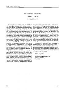
• Digital processing of a continuous-time signal involves the following basic steps: (1) Conversion of the continuous-time signal into a discrete-time signal, (2) Processing of the discrete-time signal, (3) Conversion of the processed discretetime signal back into a continuous-time signal 1

Copyright © 2010, S. K. Mitra

• Conversion of a continuous-time signal into digital form is carried out by an analog-todigital (A/D) converter • The reverse operation of converting a digital signal into a continuous-time signal is performed by a digital-to-analog (D/A) converter 2


Digital Processing of Continuos-Time Signals

• Since the A/D conversion takes a finite amount of time, a sample-and-hold (S/H) circuit is used to ensure that the analog signal at the input of the A/D converter remains constant in amplitude until the conversion is complete to minimize the error in its representation 3


• To prevent aliasing, an analog anti-aliasing filter is employed before the S/H circuit • To smooth the output signal of the D/A converter, which has a staircase-like waveform, an analog reconstruction filter is used

4


5

S/H

A/D

Digital processor

D/A

• As indicated earlier, discrete-time signals in many applications are generated by sampling continuous-time signals • We have seen earlier that identical discretetime signals may result from the sampling of more than one distinct continuous-time function

Reconstruction filter

• Since both the anti-aliasing filter and the reconstruction filter are analog lowpass filters, we review first the theory behind the design of such filters • Also, the most widely used IIR digital filter design method is based on the conversion of an analog lowpass prototype Copyright © 2010, S. K. Mitra


Sampling of Continuous-Time Signals

Complete block-diagram Antialiasing filter


6


1



• In fact, there exists an infinite number of continuous-time signals, which when sampled lead to the same discrete-time signal • However, under certain conditions, it is possible to relate a unique continuous-time signal to a given discrete-time signal 7


• If these conditions hold, then it is possible to recover the original continuous-time signal from its sampled values • We next develop this correspondence and the associated conditions

8

Effect of Sampling in the Frequency Domain


• Now, the frequency-domain representation of g a (t ) is given by its continuos-time Fourier transform (CTFT):

• Let g a (t ) be a continuous-time signal that is sampled uniformly at t = nT, generating the sequence g[n] where g [n] = g a (nT ), − ∞ < n < ∞

9

with T being the sampling period • The reciprocal of T is called the sampling frequency FT , i.e., FT = 1 T



∞

Ga ( jΩ) = ∫−∞ g a (t )e − jΩt dt • The frequency-domain representation of g[n] is given by its discrete-time Fourier transform (DTFT): − jω n G ( e jω ) = ∑ ∞ n = −∞ g[ n] e 10



Effect of Sampling in the Frequency Domain • p(t) consists of a train of ideal impulses with a period T as shown below

• To establish the relation between Ga ( jΩ) and G (e jω ) , we treat the sampling operation mathematically as a multiplication of g a (t ) by a periodic impulse train p(t): ∞

p (t ) = ∑ δ(t − nT ) n = −∞

g a (t ) 11

×

g p(t )

p (t ) Copyright © 2010, S. K. Mitra

12

• The multiplication operation yields an impulse train: ∞ g p (t ) = g a (t ) p (t ) = ∑ g a (nT )δ(t − nT ) n = −∞


2

Effect of Sampling in the Frequency Domain • g p (t ) is a continuous-time signal consisting of a train of uniformly spaced impulses with the impulse at t = nT weighted by the sampled value g a (nT ) of g a (t ) at that instant

13


Effect of Sampling in the Frequency Domain • There are two different forms of G p ( jΩ): • One form is given by the weighted sum of the CTFTs of δ(t − nT ) : − jΩnT G p ( jΩ ) = ∑ ∞ n = −∞ g a ( nT ) e • To derive the second form, we make use of the Poisson’s formula: 1 ∞ jkΩT t ∑∞ n = −∞ φ(t + nT ) = T ∑ k = −∞ Φ ( jkΩT )e where ΩT = 2π / T and Φ ( jΩ) is the CTFT 14 of φ(t ) Copyright © 2010, S. K. Mitra



• For t = 0 1 ∞ jkΩT t ∑∞ n = −∞ φ(t + nT ) = T ∑ k = −∞ Φ ( jkΩT )e

• Substituting φ(t ) = g a (t )e − jΨt in 1 ∞ ∑∞ n = −∞ φ( nT ) = T ∑ k = −∞ Φ ( jkΩT ) we arrive at 1 − jΨnT ∞ = ∑∞ ∑ n = −∞ g a (nT )e k = −∞ Ga ( j ( kΩT + Ψ ))

reduces to 1 ∞ ∑∞ n = −∞ φ( nT ) = T ∑ k = −∞ Φ ( jkΩT ) • Now, from the frequency shifting property of the CTFT, the CTFT of g a (t )e − jΨt is given by Ga ( j (Ω + Ψ )) 15


T

• By replacing Ψ with Ω in the above equation we arrive at the alternative form of the CTFT G p ( jΩ) of g p (t ) 16



• The alternative form of the CTFT of g p (t ) is given by G p ( jΩ ) = 1 T

17

• The term on the RHS of the previous equation for k = 0 is the baseband portion of G p ( jΩ) , and each of the remaining terms are the frequency translated portions of G p ( jΩ )

∞

∑ Ga ( j (Ω − kΩT ) )

k = −∞

• Therefore, G p ( jΩ) is a periodic function of Ω consisting of a sum of shifted and scaled replicas of Ga ( jΩ) , shifted by integer multiples of ΩT and scaled by 1 T



18

• The frequency range Ω Ω − T ≤Ω≤ T 2 2 • is called the baseband or Nyquist band Copyright © 2010, S. K. Mitra

3



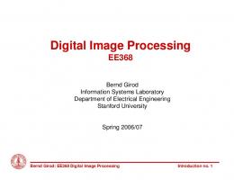
• Assume g a (t ) is a band-limited signal with a CTFT Ga ( jΩ) as shown below

• Two possible spectra of G p ( jΩ) are shown below

• The spectrum P ( jΩ) of p(t) having a sampling period T = Ω2 π is indicated below T

19


20


Effect of Sampling in the Frequency Domain If ΩT > 2Ω m , g a (t ) can be recovered exactly from g p(t ) by passing it through an ideal lowpass filter H r ( jΩ) with a gain T and a cutoff frequency Ωc greater than Ω m and less than ΩT − Ω m as shown below

• It is evident from the top figure on the previous slide that if ΩT > 2Ω m , there is no overlap between the shifted replicas of Ga ( jΩ) generating G p ( jΩ) • On the other hand, as indicated by the figure on the bottom, if ΩT < 2Ω m , there is an overlap of the spectra of the shifted replicas of Ga ( jΩ) generating G p ( jΩ) 21


22





• The spectra of the filter and pertinent signals are shown below

23


• On the other hand, if ΩT < 2Ω m , due to the overlap of the shifted replicas of Ga ( jΩ) , the spectrum Ga ( jΩ) cannot be separated by filtering to recover Ga ( jΩ) because of the distortion caused by a part of the replicas immediately outside the baseband folded back or aliased into the baseband 24


4


Effect of Sampling in the Frequency Domain • The condition ΩT ≥ 2Ω m is often referred to as the Nyquist condition • The frequency ΩT is usually referred to as 2 the folding frequency

Sampling theorem - Let g a (t ) be a bandlimited signal with CTFT Ga ( jΩ) = 0 for Ω > Ωm

• Then g a (t ) is uniquely determined by its samples g a (nT ) , − ∞ ≤ n ≤ ∞ if ΩT ≥ 2Ω m where ΩT = 2π / T 25

27


26




• Given {g a (nT )}, we can recover exactly g a (t ) by generating an impulse train g p (t ) = ∑∞ n = −∞ g a ( nT )δ(t − nT ) and then passing it through an ideal lowpass filter H r ( jΩ) with a gain T and a cutoff frequency Ωc satisfying Ω m < Ωc < (ΩT − Ω m )

• The highest frequency Ω m contained in g a (t ) is usually called the Nyquist frequency since it determines the minimum sampling frequency ΩT = 2Ω m that must be used to fully recover g a (t ) from its sampled version • The frequency 2Ω m is called the Nyquist rate


28

Effect of Sampling in the Frequency Domain • Oversampling - The sampling frequency is higher than the Nyquist rate • Undersampling - The sampling frequency is lower than the Nyquist rate • Critical sampling - The sampling frequency is equal to the Nyquist rate • Note: A pure sinusoid may not be recoverable from its critically sampled version 29 Copyright © 2010, S. K. Mitra


Effect of Sampling in the Frequency Domain • In digital telephony, a 3.4 kHz signal bandwidth is acceptable for telephone conversation • Here, a sampling rate of 8 kHz, which is greater than twice the signal bandwidth, is used

30


5

Effect of Sampling in the Frequency Domain • In high-quality analog music signal processing, a bandwidth of 20 kHz has been determined to preserve the fidelity • Hence, in compact disc (CD) music systems, a sampling rate of 44.1 kHz, which is slightly higher than twice the signal bandwidth, is used 31


Effect of Sampling in the Frequency Domain • Example - Consider the three continuoustime sinusoidal signals: g1(t ) = cos(6πt ) g 2 (t ) = cos(14πt ) g3 (t ) = cos(26πt ) • Their corresponding CTFTs are: G1( jΩ) = π[δ(Ω − 6π) + δ(Ω + 6π)] G2 ( jΩ) = π[δ(Ω − 14π) + δ(Ω + 14π)] G3 ( jΩ) = π[δ(Ω − 26π) + δ(Ω + 26π)] 32




• These three transforms are plotted below

• These continuous-time signals sampled at a rate of T = 0.1 sec, i.e., with a sampling frequency ΩT = 20π rad/sec • The sampling process generates the continuous-time impulse trains, g1 p (t ) , g 2 p (t ) , and g3 p (t ) • Their corresponding CTFTs are given by 33


34





• Plots of the 3 CTFTs are shown below

35

Glp ( jΩ) = 10∑∞ k = −∞ Gl ( j (Ω − kΩT ) ), 1 ≤ l ≤ 3

36

• These figures also indicate by dotted lines the frequency response of an ideal lowpass filter with a cutoff at Ωc = ΩT / 2 = 10π and a gain T = 0.1 • The CTFTs of the lowpass filter output are also shown in these three figures • In the case of g1(t ), the sampling rate satisfies the Nyquist condition, hence no aliasing Copyright © 2010, S. K. Mitra

6



• Note: In the figure at the bottom, the impulse appearing at Ω = 6π in the positive frequency passband of the filter results from the aliasing of the impulse in G2 ( jΩ) at Ω = −14π • Likewise, the impulse appearing at Ω = 6π in the positive frequency passband of the filter results from the aliasing of the impulse in G3 ( jΩ) at Ω = 26π

• Moreover, the reconstructed output is precisely the original continuous-time signal • In the other two cases, the sampling rate does not satisfy the Nyquist condition, resulting in aliasing and the filter outputs are all equal to cos(6πt) 37


38



• We now derive the relation between the DTFT of g[n] and the CTFT of g p (t ) • To this end we compare − jω n G ( e jω ) = ∑ ∞ n = −∞ g[ n] e with − jΩnT G p ( jΩ ) = ∑ ∞ n = −∞ g a ( nT ) e

• Observation: We have G ( e jω ) = G p ( jΩ ) Ω =ω / T or, equivalently, G p ( jΩ ) = G ( e jω ) ω=ΩT • From the above observation and

G p ( jΩ ) = 1

and make use of g[ n] = g a (nT ), − ∞ < n < ∞

39


T

40

we arrive at the desired result given by ∞

=1 T

k = −∞ ∞

Ω =ω / T

∑ Ga ( j Tω − jkΩT )

k = −∞ ∞

= 1 ∑ Ga ( j ω − j 2 π k ) T T T k = −∞

41


∞

∑ Ga ( j (Ω − kΩT ) )

k = −∞



Effect of Sampling in the Frequency Domain G (e jω ) = T1 ∑ Ga ( jΩ − jkΩT )


42

• The relation derived on the previous slide can be alternately expressed as G (e jΩT ) = T1 ∑∞ k = −∞ Ga ( jΩ − jkΩT ) • From G ( e jω ) = G p ( jΩ ) Ω =ω / T or from G p ( jΩ ) = G ( e jω ) ω=ΩT it follows that G (e jω ) is obtained from Gp ( jΩ) by applying the mapping Ω = ω T Copyright © 2010, S. K. Mitra

7


Recovery of the Analog Signal • We now derive the expression for the output g^ a (t ) of the ideal lowpass reconstruction filter H r ( jΩ) as a function of the samples g[n] • The impulse response hr (t ) of the lowpass reconstruction filter is obtained by taking the inverse DTFT of H r ( jΩ): T , Ω ≤ Ωc H r ( jΩ) = ⎧⎨ ⎩ 0, Ω > Ωc

• Now, the CTFT Gp ( jΩ) is a periodic function of Ω with a period ΩT = 2π / T • Because of the mapping, the DTFT G (e jω ) is a periodic function of ω with a period 2π

43


Recovery of the Analog Signal

• Thus, the impulse response is given by

• Therefore, the output g^ a (t ) of the ideal lowpass filter is given by:

1 ∞ H ( jΩ) e jΩt dΩ = T Ω c e jΩt dΩ 2 π −∞ r 2 π −Ωc

∫

∫

sin(Ωct ) , −∞ ≤t ≤ ∞ = ΩT t / 2 • The input to the lowpass filter is the impulse train gp(t ) : g p (t ) = ∑∞ n = −∞ g[ n] δ(t − nT )


g^ a (t ) = hr (t ) * g p (t ) =

n = −∞

Recovery of the Analog Signal • It can be shown that when Ωc = ΩT / 2 in sin( Ω ct ) hr (t ) =

• The ideal bandlimited interpolation process is illustrated below


∞

∑ g[n]hr (t − nT )

• Substituting hr (t ) = sin(Ωct ) /(ΩT t / 2) in the above and assuming for simplicity Ωc = ΩT / 2 = π / T , we get ∞ sin[ π(t − nT ) / T ] ^ (t ) = g g[ n] ∑ a 46 π(t − nT ) Copyright / T © 2010, S. K. Mitra n = −∞

Recovery of the Analog Signal

47


Recovery of the Analog Signal hr (t ) =

45

44

ΩT t / 2

h r(0) = 1 and h r(nT ) = 0 for n ≠ 0 • As a result, from sin[ π(t − nT ) / T ] g^ a (t ) = ∑∞ n = −∞ g[ n] π(t − nT ) / T we observe g^ a (rT ) = g[ r ] = g a (rT ) 48

for all integer values of r in the range −∞ < r < ∞ Copyright © 2010, S. K. Mitra

8

Implication of the Sampling Process

Recovery of the Analog Signal • The relation g^ a (rT ) = g[ r ] = g a (rT )

• Consider again the three continuous-time signals: g1(t ) = cos(6πt ) , g 2 (t ) = cos(14πt ) , and g3 (t ) = cos( 26πt ) • The plot of the CTFT G1p ( jΩ) of the sampled version g1p (t ) of g1 (t ) is shown below

holds whether or not the condition of the sampling theorem is satisfied • However, g^a (rT ) = g a (rT ) for all values of t only if the sampling frequency ΩT satisfies the condition of the sampling theorem 49

51


50



• From the plot, it is apparent that we can recover any of its frequency-translated versions cos[(20k ± 6)π t] outside the baseband by passing g1p (t ) through an ideal analog bandpass filter with a passband centered at Ω = (20k ± 6)π

• For example, to recover the signal cos(34πt), it will be necessary to employ a bandpass filter with a frequency response


0.1, (34 − Δ)π ≤ Ω ≤ (34 + Δ )π H r ( jΩ) = ⎧⎨ otherwise ⎩ 0, where Δ is a small number

52





• Likewise, we can recover the aliased baseband component cos(6πt) from the sampled version of either g 2 p (t ) or g3 p (t ) by passing it through an ideal lowpass filter with a frequency response: 0.1, (6 − Δ )π ≤ Ω ≤ (6 + Δ )π H r ( jΩ) = ⎧⎨ otherwise ⎩ 0, 53


• There is no aliasing distortion unless the original continuous-time signal also contains the component cos(6πt) • Similarly, from either g 2 p (t ) or g3 p (t ) we can recover any one of the frequencytranslated versions, including the parent continuous-time signal g 2(t ) or g3(t ) as the case may be, by employing suitable filters 54


9

Sampling of Bandpass Signals


• The conditions developed earlier for the unique representation of a continuous-time signal by the discrete-time signal obtained by uniform sampling assumed that the continuous-time signal is bandlimited in the frequency range from dc to some frequency Ωm

• There are applications where the continuoustime signal is bandlimited to a higher frequency range Ω L ≤ Ω ≤ Ω H with Ω L > 0 • Such a signal is usually referred to as the bandpass signal • To prevent aliasing a bandpass signal can of course be sampled at a rate greater than twice the highest frequency, i.e. by ensuring ΩT ≥ 2Ω H

• Such a continuous-time signal is commonly referred to as a lowpass signal 55


56



• However, due to the bandpass spectrum of the continuous-time signal, the spectrum of the discrete-time signal obtained by sampling will have spectral gaps with no signal components present in these gaps • Moreover, if Ω H is very large, the sampling rate also has to be very large which may not be practical in some situations

• A more practical approach is to use undersampling • Let ΔΩ = Ω H − Ω L define the bandwidth of the bandpass signal • Assume first that the highest frequency Ω H contained in the signal is an integer multiple of the bandwidth, i.e., Ω H = M (ΔΩ)

57


58

• This leads to ( ) G p ( jΩ ) = 1 ∑ ∞ k = −∞ Ga jΩ − j 2k (ΔΩ)

• We choose the sampling frequency ΩT to satisfy the condition 2Ω ΩT = 2(ΔΩ) = H M which is smaller than 2Ω H , the Nyquist rate • Substitute the above expression for ΩT in G p ( jΩ ) = 1 T

T

• As before, G p( jΩ) consists of a sum of Ga( jΩ) and replicas of Ga( jΩ) shifted by integer multiples of twice the bandwidth ΔΩ and scaled by 1/T • The amount of shift for each value of k ensures that there will be no overlap between all shifted replicas no aliasing

∞

∑ Ga ( j (Ω − k ΩT ))

k = −∞





59


60


10

Sampling of Bandpass Signals • Figure below illustrate the idea behind Ga ( jΩ)

− ΩH − ΩL

0

ΩL

ΩH

ΩL

ΩH

Ω

G p ( jΩ )

− ΩH − ΩL

61

0

Ω


Sampling of Bandpass Signals • As can be seen, g a (t ) can be recovered from g p (t ) by passing it through an ideal bandpass filter with a passband given by Ω L ≤ Ω ≤ Ω H and a gain of T • Note: Any of the replicas in the lower frequency bands can be retained by passing g p (t ) through bandpass filters with passbands Ω L − k ( ΔΩ) ≤ Ω ≤ Ω H − k (ΔΩ) , 1 ≤ k ≤ M − 1 providing a translation to lower frequency ranges 62 Copyright © 2010, S. K. Mitra

11

Digital Processing of Continuous-Time Signals Digital ... - yarbis

Digital Processing of Continuous-Time Signals Digital ... - yarbis

Suggest Documents

Digital Signal Processing the Tevatron BPM Signals

Digital Signal Processing applied to Physical Signals

Digital Image Processing (Digital bildbehandling grundkurs) Digital ...

Lab 1 -- Digital Signals

digital processing of speech and image signals - Www I6 Informatik ...

digital processing of speech signals (rabiner & schafer 1978).pdf ...

digital processing of speech signals (rabiner & schafer 1978).pdf ...

audio signals processing with digital filters ... - ARPN Journals

Digital Image Processing 2. Digital Image Fundamentals

LabVIEW Digital Signal Processing and Digital Communications

Digital Image Processing Digital Image Processing - CPE, KU

Digital Signal Processing

Digital Speech Processing

Digital Image Processing

DIGITAL IMAGE PROCESSING: APPLICATIONS

Digital Image Processing - ImageProcessingPlace

digital signal processing

Digital Image Processing - MAFIADOC.COM

Digital Image Processing - ImageProcessingPlace

Advanced Digital Signal Processing

Digital Signal Processing

Digital Image Processing - DCC

BIOMEDICAL DIGITAL SIGNAL PROCESSING

Digital Signal Processing