Language enhanced with External Authoring Interface for visualization and ... Just as maps can visually enhance the spatial understanding of phenomena,.
Digital Soil Mapping - An Introductory Perspective P. Lagacherie, A.B. McBratney and M. Voltz (eds.) Elsevier Publisher - Developments in Soil Science Series
Chapter 43: Are Current Scientific Visualization and Virtual Reality Techniques Capable to Represent Real Soil-Landscapes?
S. Grunwald, V. Ramasundaram, N.B. Comerford and C.M. Bliss
Abstract Real soil-landscapes are complex consisting of an inextricable mix of patterns and noise varying continuously in the space-time continuum. Soils and parent material show gradual variations in the horizontal and vertical planes forming 3D bodies that are commonly anisotropic. There is no real beginning and end point in soil-landscapes because environmental conditions are dynamically changed through water flow, biogeochemical processes, and human activities. The strengths of soil-landscape modeling lies in hypothesis testing, understanding causal linkages between environmental factors, and their interrelationships within a spatial and temporal explicit context. To develop virtual soil-landscape models entails: (i) conceptualization, i.e. defining the model framework (e.g. finite space elements) (ii) reconstruction, i.e. describing and quantifying underlying conditions and behavior and (iii) scientific visualization (SciVis), i.e. abstracting real soil-landscapes into a format that we can comprehend and that helps us to understand the complexity of soil-landscapes. The primary objective in data visualization is to gain insight into an information space by mapping data onto graphical primitives. Capabilities and limitations of SciVis and virtual reality techniques are discussed in this chapter. Only recently 3D soillandscape models have been emerging. We present a case study that translated the spatiotemporal water table dynamics of a flatwood soil-landscape in Florida into a virtual domain using a geostatistical method to reconstruct the soil-landscape and Virtual Reality Modeling Language enhanced with External Authoring Interface for visualization and implementation of interactive functions. Just as maps can visually enhance the spatial understanding of phenomena, interactive spatio-temporal applications can enhance our understanding of complex environmental systems and the underlying transport processes driving soil and water quality.
43.1 Introduction Scientists have focused on two contrasting concepts to study soil-landscapes and ecosystem processes which are both equally important. The reductionist approach promotes ever more detailed studies of distributions, soil classes, events and processes, followed by their interpretation. The other approach develops and enunciates an integrative, unifying point of view encompassing and integrating previous observations and results. Both concepts have been employed for quantitative spatially explicit modeling of soil forming factors evolving through time.
Different kinds of models have been used to translate real soil-landscapes and ecosystem processes into virtual environments. Hoosbeek and Bryant (1994) provide an overview of pedological models using criteria such as the relative degree of computation (qualitative vs. quantitative models), complexity of the model structure (functional vs. mechanistic models) and level of organization (soil region, pedon to molecular scale). Modeling is about choosing the appropriate metaphor or analogy with which to better understand a phenomenon, e.g. the spatial distribution of soils, their behavior and relationship to other environmental factors. In this sense, we create media about phenomena to bridge the gap between what we do not know, and what we are trying to comprehend. Media such as slides, maps, animations, three-dimensional (3D) virtual worlds, and digital libraries are also models. Although one might talk of absolutes such as “reality” and “truth”, all we have at our disposal are models, which mediate the world for us. We have to acknowledge that different media have different effects on our understanding and interpretation of objects, such as soil-landscapes and ecosystem processes. The following criteria potentially influence to transcend real into virtual soil-landscapes: (i) space, (ii) time, (iii) scale,
(iv) ecosystem condition, (v) spatial and temporal variability (vi) interrelationships between environmental factors and (vii) causal linkages or behavior of the system.
The modeling process can be disaggregated into: (i) conceptualization, i.e. defining the model framework (e.g. finite space elements) (ii) reconstruction, i.e. describing and quantifying underlying conditions and behavior and (iii) scientific visualization (SciVis), i.e. abstracting real soil-landscapes into a format that we can comprehend and that helps us to understand the complexity of soil-landscapes.
Scientific visualization is defined as the use of the human visual processing system assisted by computer graphics, as a means for the direct analysis and interpretation of information. McCormick et al. (1987) indicated that SciVis transforms the symbolic into the geometric, enabling researchers to observe their simulations and computations. It offers a method for seeing the unseen. It enriches the process of scientific discovery and fosters profound and unexpected insights. In many fields it is already revolutionizing the way scientists do science (McCormick et al., 19987). Senay and Ignatius (1994) point out that the primary objective in data visualization is to gain insight into an information space by mapping data onto graphical primitives.
Real soil-landscapes are complex consisting of an inextricable mix of patterns and noise varying continuously in the space-time continuum. Soils and parent material show gradual variations in the horizontal and vertical planes forming 3D bodies that are commonly anisotropic. There is no real beginning and end point in real soil-landscapes because environmental
conditions are dynamically changed through water flow and biogeochemical processes. In addition, human induced changes have had remarkable effects on almost all soil-landscapes.
Transforming real into virtual soil-landscapes is based on model predictions and estimations both associated with uncertainty. Estimations use sample data to make an inference about a population whereas prediction refers to a statement made about the future or reasoning about the future. Methods used in science for the derivation of predictions of unknown facts from known facts include (modified after Bunge, 1959): (1) Logical inference entailing deduction, induction and abduction, the latter one referring to the generation of hypotheses to explain observations (2) Structural laws help predict new properties from the known properties of material or formal structures (3) Phenomenological laws predict phenomena on the basis of known constant associations (4) Functional laws infer properties of a system from knowledge of the functional role of the parts and their interconnections (5) Statistical laws help derive collective properties of classes of events from an analysis of such classes (6) Mechanical laws extrapolate future (or past) states on the basis of known current states and relations (e.g. Newtonian laws).
43.1.1 Time and space concepts Frank (1998) and Raper (2000) provide an overview of time models. Almost all existing soil-landscape models are based on Newtonian time that is focused on a succession of
phenomena along a linear time coordinate providing the simplest time concept characterized by causal inertness. Time is viewed as a neutral framework against which independently unfolding events are projected, sorted and measured. Newton argued that time is absolute implying that the universe has a single universal clock capable of determining that two occurrences are simultaneously. The present moment forms the center point changing constantly. Backcasting and forecasting models exists predicting past and future events (e.g. formation of Spodosols, land use change models) with exponentially increasing prediction errors from the present moment. Other soil-landscape models are “snapshot models” that are limited to describe current environmental conditions. Characteristics of “real” time include that events are non-repeatable and sometimes structured and at other times chaotic.
Generally, it is necessary to divide geographical space into discrete spatial units and the resulting tessellation is taken as a reasonable approximation of reality at the level of resolution under consideration (Burrough and McDonnell, 1998). There are two types of spatial discretization methods used for soil-landscape modeling: (i) crisp soil map units and (ii) the continuous fields model or pixel-based model (Peuquet, 1988; Goodchild, 1992; Burrough and McDonnell, 1998). The crisp model has its roots in empiric observations combined with 19th century biological taxonomy and practice in geological survey. Traditional soil-landscape models use crisp map units which are defined by abrupt changes from one map unit to the other (Voltz and Webster, 1990; Webster and Oliver, 1990). Each soil map unit is associated with a representative soil attribute set (Soil Survey Staff, 1998). Horizons of these soil map units differ from adjacent and genetically related layers in physical, chemical, morphological and biological properties such as texture, structure, color, soil organic matter, or degree of acidity. As such, soil
horizons and profiles of these properties correspond to discrete, sharply delineated (crisp) units, which are assumed to be internally uniform. The crisp soil model has been questioned and critically discussed repeatedly (Webster and De La Cuanalo, 1975; Nortcliff, 1978; Nettleton et al, 1991; McBratney and de Gruijter, 1992; Heuvelink and Webster, 2001). An alternative geographic model displays the real world as a set of pixels or voxels (volume element) and is adequate for modeling natural phenomena that do not show obvious boundaries (e.g. soils). This spatial model has the potential to describe the gradual change of soil properties formed by a variety of pedological processes within a domain. The spatial resolution depends on the spatial variability of soil properties. Geostatistical techniques have been introduced to interpolate point observations and construct soil property pixel maps (Goovaerts, 1997; Chilès and Delfiner, 1999; Webster and Oliver, 2001). Challenging is to optimize the density and spatial distribution of observations across a domain to characterize soil-landscape reality without knowing the real spatial distribution of soil properties and operating pedological processes. Crisp and the pixel model have been used extensively to produce two-dimensional soil maps. This contradicts with the conceptual view of soils as 3D natural bodies. McSweeney et al. (1994) proposed a 3D framework for soil-landscape modeling that has yet to be adopted by soil surveyors and pedologists.
43.1.2 Are current quantitative reconstruction techniques capable to capture spatial and temporal variability of properties and behavior? The strengths of soil-landscape modeling lies in hypothesis testing, understanding causal linkages between environmental factors, and their interrelationships within a spatial and temporal
explicit context. Goovaerts (1999), McBratney et al. (2000), Heuvelink and Webster (2001), McBratney et al. (2003) and Grunwald (2005) provided a comprehensive overview of pedometric techniques to model soil spatial and temporal variation. Advanced modeling techniques exist; yet there are major limitations that prohibit their widespread adoption. Geostatistical methods are data intensive requiring a large number of point observations (Webster and Oliver, 2001). Similarly dense frequency datasets are required to describe the change of soil and environmental properties through time. In short, geo-temporal modeling of soil-landscapes is data intensive. Process-based mechanistic models offer alternatives to simulate soil-landscape evolution through time (Minasny, 1999). However, most pedological processes operate over long time periods. For those reasons it is challenging to validate pedodynamic process models. Emerging soil mapping techniques (e.g. soil sensors, remote sensors) provide new opportunities to collect exhaustive datasets that support the reconstruction of soillandscapes. Yet uncertainties of such datasets are typically high constraining their use.
43.1.3 Are current scientific visualization and virtual reality techniques capable to represent real soil-landscapes? The Internet, geographic information technology, and SciVis provide new education and information delivery capabilities. Numerous studies have shown that SciVis is effective for enhancing rote memorization and higher-order cognitive skills (Koussoulakou and Kraak, 1992; Barraclough and Guymer, 1998). Stibbard (1997) found that information is absorbed best when using more than one human sense; i.e., 10% of the information is taken in by reading, 30% by reading and visual, 50% by reading, visuals and sound, 80% by reading, visuals, sound and
interaction. Koussoulakou and Kraak (1992) tested the usefulness of different SciVis methods including static maps, series of static maps, and animated maps, and found significantly better response times for animated maps. Barraclough and Guymer (1998) reported that advanced visualization techniques served to better communicate spatial information between people in different fields, such as scientists, administrators, educators, and the general public. Just as maps can visually enhance the spatial understanding of phenomena, interactive spatio-temporal applications can enhance our understanding of complex environmental systems and the underlying transport processes driving soil and water quality. According to Fisher and Unwin (2002) visual interfaces maximize our natural perception abilities, improve to comprehend huge amounts of data, allow the perception of emergent properties that were not anticipated, and facilitate understanding of both large-scale and small-scale geographic features of ecosystems.
Only recently 3D soil-landscape models have been emerging. For example, a 3D soil horizon model in a Swiss floodplain was created by Mendonça Santos et al. (2000) using a quadratic finite-element method. Grunwald et al. (2000) presented 3D soil-landscape models at different scales for sites in southern Wisconsin using Virtual Reality Modeling Language (VRML). Sirakow and Muge (2001) developed a prototype 3D Subsurface Objects Reconstruction and Visualization System (3D SORS) in which 2D planes are used to assemble 3D subsurface objects.
The development of immersive and desktop virtual reality (VR) techniques has been instrumental to develop virtual soil-landscapes and environments. VRML-based models enhanced with Java and External Authoring Interface provide capabilities to display real soil-
landscapes in 3D and 4D digital formats (Ramasundaram et al., 2004). Characteristics of VR include: (i) immersion, (ii) navigation (freedom for the user to explore) and (iii) interaction. Virtual reality applications are still limited to prototype applications and have not found widespread adoption. Reasons that constrain the extended production of virtual soil-landscape models are due to (i) input data requirements, (ii) labor intensive production (programming is required), (iii) lack in training and education of people to produce such models, (iv) preference of users for traditional 2D maps and (v) lack of realistic abstraction of real soil-landscapes.
43.2 Case study Our goal was to translate a real into a virtual soil-landscape in Florida. We discuss the limitations of our approach in context of conceptualization, reconstruction and SciVis.
43.2.1 Objectives Specific objectives were (i) to reconstruct a flatwood soil-landscape in Florida to describe and display the spatial distribution of soils and topography in 3D format and (ii) to develop space-time simulations that describe and display water flow in four-dimensional (4D) format.
43.2.2 Methodology The study area comprised a 42-ha site in northeastern Florida with hydric and non-hydric soils. About one third of the site was covered by bald cypress (Taxodium distichum) and about two-thirds by slash pine (Pinus elliottii). In 1994, three silvicultural treatments were
administered. While one area was left as a control (uncut), a second area was clearcut. In the third area only the forest on the hydric soils was cut and that on the non-hydric soils left untouched. Morphological and taxonomic soil data were collected at 123 locations. Water table was monitored biweekly at 123 wells from April 1992 to March 1998. Topography was characterized by laser level and ranged from 26.7 to 30.8 meters.
We developed a model that characterizes soil horizons and terrain across the flatwood site. A digital elevation model (DEM) was developed using the observed point elevation values and ordinary kriging. Soil horizon depths were interpolated in the horizontal plane using ordinary kriging and linear interpolation in the vertical plane to create soil volumes representing the horizons. Virtual Reality Modeling Language was used to render face geometry of the soil horizon model (Lemay et al., 1999) and fuse the DEM and soil horizons. The IndexedFaceSet VRML class was employed to render polyhedrons. A point-arc geographic data model was used to create IndexFaceSets. The appearance of volume objects was coded using the RGB (red-greeblue) color classification system. An interface is necessary to communicate between a VRML world and an external environment. This interface is called an External Authoring Interface (EAI) and it defines the set of functionality of the VRML web browser that the external environment can access. To add interactivity to our web-based model we developed a Java applet to extend the capability of the Blaxxun3D Java applet, which supports the VRML Java EAI interface.
Dynamic models of hydropatterns were developed from precipitation data and water table measurements for a period of 6 years (April 1992 and March 1998) using 15-day time
increments. Hundreds of semivariograms for water table depth had to be generated, each representing one specific time period. Water table levels were interpolated using ordinary kriging. The water table surface was sliced with the DEM to distinguish inundated from noninundated areas. The CoordinateInterpolator VRML node was used to produce a smooth display of water table depths between observation periods. Water inundation models for each time period were stored in a digital library. The IndexedFaceSet VRML class was employed to render the extent of the study site. The graphical user interface was implemented using a Java Applet that reads the models on-the-fly from the digital library constraint by user-defined start and end times for a inundation simulation.
43.2.3 Results and discussion The 3D soil horizon model infused with a DEM is shown in Fig. 1 and a demo is available at http://3dmodel.ifas.ufl.edu. To access the model a web browser and VRML plug-in such as Blaxxun3D are required. Users have the ability to view the whole model or each soil horizon independently. VRML sensors enable to rotate, zoom, tilt or pan the model giving users the feeling of emergence in the web-based world. Soil horizons are displayed continuously in 3D geographic space taking into account the displacement from the soil surface.
We implemented the space-time simulations of water table dynamics in an interactive framework. Users can trigger an event (e.g. inundation simulation) by constraining the border conditions (e.g. time period, geographic domain) of simulations interactively (Fig. 2). Such an adaptive simulation framework invites users to study water table dynamics through observations
using a sequence of events: trigger an event – observe ecosystem process – interpretation – assimilation.
Users can study the expansion and contraction of inundated areas over time. This implementation is dynamic and superior when compared to a static 2D GIS “snapshot” map that shows water tables at few specific times. Though elevation changes across the study area are small topography is the major factor driving water table dynamics on this flatwood site. The upslope drainage area defined the amount of surface water (and most likely some shallow lateral water) draining into the depressional areas. Spodosols and their distinct horizons confounded water flow driven by surface terrain.
We considered the following criteria for the development of our model-simulation environment: (i) Global access, i.e., web-based implementation, (ii) Simulation of a variety of learning mechanisms, (iii) Interactivity to engage users, (iv) Compartmentalization and hierarchical organizational structure, (v) Abstraction of 2D and 3D geographic objects (e.g. soils, terrain) and dynamic ecosystem processes (e.g. water flow) using geostatistics and SciVis techniques. We used a relatively simple reconstruction method (ordinary kriging) because hundreds of variograms and kriged models needed to be produced. However, in this study we focused on SciVis to gain a better understanding of water table dynamics at the soil-terrain interface over a long period of time.
Our dataset was unique covering a long time-period with dense observations in time and space. We were able to visualize causal linkages between terrain properties, land use, soils and
water movement within a spatial and temporal explicit context. Employing SciVis facilitated multiple views of the content world, which stimulates a greater understanding and insight of the flatwood system. It is this synthesis of geographic datasets that distinguishes the virtual learning environment from conventional instructional media (e.g 2D GIS maps). The availability of multiple representations - maps, 3D models, space-time models, text - of the same geographical region, each of which offers a different perspective of the soil-landscape, has the potential to improve our understanding of flatwood water dynamics. Desktop virtual reality when combined with other forms of digital media may offer great potential for a cognitive approach to research and education. Scientific visualization combined with quantitative reconstruction techniques has the potential to translate soil-landscapes and ecosystem processes into a transparent format to enhance our understanding of real-world phenomena and complex environmental systems. Virtual soil-landscape models are beneficial in disseminating geo-referenced soil and landscape data to educators, researchers, government agencies, and the general public.
Acknowledgement All the information concerning the research area was collected by C.M. Bliss and N.B. Comerford. We also thank the National Council for Air and Stream Improvement (NCASI) and US Forest Service for funds that allowed the data collection as well as Rayonier, Inc. for allowing the study on their land. We also thank Adrien Mangeot for parts of the coding. This research was supported by the Florida Agricultural Experiment Station and approved for publication as Journal Series No. R-10877.
References Barraclough, A. and Guymer, I., 1998. Virtual reality – a role in environmental engineering education? Water Sci. Tech., 38(11): 303-310.
Bunge, M., 1959. Causality. Mass. Harward University Press, Cambridge.
Burrough, P.A. and McDonnell, R. A., 1998. Principles of Geographical Information Systems. Oxford University Press, New York.
Chilès, J.-P. and Delfiner, P., 1999. Geostatistics – Modeling Spatial Uncertainty. John Wiley & Sons, New York.
Fisher, P. and Unwin, D., 2002. Virtual reality in geography. Taylor & Francis, New York.
Frank, A.U., 1998. Different types of “times” in GIS. In Egenhofer m.J. and R.G. Golledge (eds.) Spatial and Temporal Reasoning in Geographic Information Systems. Oxford University Press, New York.
Goodchild, M., Sun, G. and Yang, S., 1992. Development and test of an error model for categorical data. Int. J. of Geographical Information Systems, 6 (2): 87-104.
Goovaerts, P., 1997. Geostatistics for Natural Resources Evaluation. Oxford University Press, New York.
Goovaerts, P., 1999. Geostatistics in soil science: state-of-the-art and perspectives. Geoderma, 89: 1-45.
Grunwald, S., Barak, P., McSweeney, K. and Lowery, B., 2000). Soil landscape models at different scales portrayed in Virtual Reality Modeling Language. J. of Soil Science, 165(8): 598-615.
Grunwald S. (2005) (eds.) Environmental Soil-Landscape Modeling. CRC Press, New York.
Heuvelink G.B.M. and Webster R. 2001. Modeling soil variation: past, present, and future. Geoderma 100: 269-301.
Hoosbeek, M.R. and Bryant, R.B., 1994. Developing and adapting soil process submodels for use in the pedodynamic Orthod model. In Bryant R.B and R.W. Arnold (eds.) Quantitative Modeling of Soil Forming Processes, SSSA Special Publ. No. 39, Madison, WI, USA.
Lemay, L., Couch, J. and Murdock, K., 1999.3D graphics and VRML 2. Sams.net Publ., Indianapolis, IN.
Koussoulakou, A. and Kraak, M.J., 1992. Spatio-temporal maps and cartographic communication. Cartographic J. 29, 101-108.
McBratney, A.B. and de Grujiter, J.J., 1992. A continuum approach to soil classification by modified fuzzy k-means with extragrades. J. of Soil Science, 43: 159-175.
McBratney, A.B., Odeh, I.O.A., Bishop, T.F.A., Dunbar, M.S. and Shatar, T.M., 2000. An overview of pedometric techniques for use in soil survey. Geoderma, 97: 293-327.
McBratney, A.B., Mendonca Santos, M.L. and Minasny, B., 2003. On digital soil mapping. Geoderma, 117: 3-52.
McCormick, B.H., DeFanti, T.A. and Brown, M.D. (eds.). 1987. Visualization in scientific computing. Computer Graphics 21(6), (entire issue).
McSweeney, K., Gessler, P.E., Slater B.K., Hammer, R.D., Peterson, G.W. and Bell, J.C., 1994. Towards a new framework for modeling the soil-landscape continuum. SSSA Special Publ. 33, Factors in Soil Formation.
Mendonça Santos, M.L., Guenat, C., Bouzelboudjen, M. and Golay, F., 2000. Three-dimensional GIS cartography applied to the study of the spatial variation of soil horizons in a Swiss floodplain. Geoderma, 97: 351-366.
Minasny, B. and McBratney, A.B., 1999. A rudimentary mechanistic model for soil production and landscape development. Geoderma, 90: 3-21.
Nettleton, W.D., Brasher, B.R. and Borst, G., 1991. The taxadjunct problem. Soil Sci. Soc. Am. J., 55: 421-427.
Nortcliff, S. 1978. Soil variability and reconnaissance soil mapping: A statistical study in Norfolk. J. Soil Science, 29: 403-418.
Peuquet, D., 1988. Presentations of geographic space: towards a conceptual synthesis. Annals of the Association of American Geographers, 78 (3): 375-394.
Ramasundaram, V., Grunwald, S., Mangeot, A., Comerford, N.B. and Bliss, C.M., 2004. Development of an environmental virtual field laboratory. Computers & Education J. 45: 21-34.
Raper, J., McCarthy, T. and Williams, N., 1998. Georeferenced four-dimensional virtual environments: principles and applications. Computers, Environment and Urban Systems, 22(6): 529-539.
Senay, H. and Ignatius, E., 1994. A knowledge-based system for visualization design. IEEE Computer Graphics and Applications: 36-47.
Sirakov, N.M. and Muge, F.H., 2001. A system for reconstructing and visualizing threedimensional objects. Computers & Geosciences, 27: 59-69.
Stibbard A. 1997, Warwick University Forum, No. 6.
Soil Survey Staff. 1998. Keys to soil taxonomy, 8th Ed. Govt. Printing Office, Washington, DC.
Voltz M and Webster R. 1990. A comparison of kriging, cubic splines and classification for predicting soil properties from sample information. J. Soil Science 31: 505-524.
Webster, R. and De La Cuanalo, H.E., 1975. Soil transect correlograms of North Oxfordshire and their interpretation. J. Soil Science, 26: 176-194.
Webster, R. and Oliver, M.A., 1990. Statistical methods in soil and land resource survey, Oxford University Press, Oxford.
Webster, R. and Oliver, M.A. 2001. Geostatistics for Environmental Scientists. John Wiley & Sons, Chichester, England.
Figure captions Fig. 43.1. Soil horizon model infused with a DEM representing a Florida flatwood site. Fig. 43.2. Three snapshots of simulations of inundated areas at different time periods.
Fig. 43.1.
Fig. 43.2.