Diluted three-dimensional random field Ising model at zero ... - Core

PHYSICAL REVIEW B 74, 104409 共2006兲

Diluted three-dimensional random field Ising model at zero temperature with metastable dynamics Xavier Illa* and Eduard Vives† Departament d’Estructura i Constituents de la Matèria, Martí i Franquès 1, Facultat de Física, Universitat de Barcelona, 08028 Barcelona, Catalonia, Spain 共Received 12 May 2006; revised manuscript received 21 June 2006; published 11 September 2006兲 The influence of vacancy concentration on the behavior of the three-dimensional random field Ising model with metastable dynamics is studied. We have focused our analysis on the number of spanning avalanches which allows us a clear determination of the critical line where the hysteresis loops change from continuous to discontinuous. By a detailed finite-size scaling analysis we determine the phase diagram and numerically estimate the critical exponents along the whole critical line. Finally, we discuss the origin of the curvature of the critical line at high vacancy concentration. DOI: 10.1103/PhysRevB.74.104409

PACS number共s兲: 75.50.Lk, 75.40.Mg, 05.50.⫹q, 75.10.Nr

I. INTRODUCTION

Externally driven systems at sufficiently low temperature often display rate-independent hysteresis. This out-ofequilibrium phenomenon occurs because intrinsic disorder creates multiple energy barriers that the system cannot overcome due to very weak thermal fluctuations. The study of zero-temperature models with metastable dynamics has been very successful for understanding rateindependent hysteresis. A prototypical case is the random field Ising model 共RFIM兲 with single spin-flip relaxation dynamics.1,2 Although the model is formulated in terms of magnetic variables 共external field H and magnetization m兲, it can be applied to the study of many phenomena associated with low-temperature first-order phase transitions in disordered systems, e.g., martensitic transformations,3 fluid adsorption in porous solids,4 ferroelectrics,5 etc. Disorder is an intriguing concept; in the RFIM it is introduced via independent, quenched random fields on each lattice site, Gaussian-distributed with zero mean, and standard deviation ␴. In real materials, disorder is much more complicated and includes features on all length scales: vacancies, interstitials, composition fluctuations, dislocations, strain fields, grain boundaries, sample surfaces, edges and corners, etc. Thus, it is interesting to add to the RFIM other sources of disorder, in order to see how nonequilibrium behavior is modified. The goal of this paper is to study the diluted RFIM at T = 0 with metastable dynamics and to analyze the consequence of introducing a concentration c of quenched vacancies. The interplay between the two kinds of disorder 共random fields and vacancies兲 will be at the origin of the properties of the ␴-c phase diagram. One of the striking results concerning the RFIM with metastable dynamics, as already pointed out in the seminal paper of Sethna et al.,1 is the occurrence of a critical point when the amount of disorder ␴ is increased. The m vs H hysteresis loops change from being discontinuous 共as in a ferromagnet兲 when ␴ ⬍ ␴c to continuous 共as in a spin glass兲 when ␴ ⬎ ␴c. This result was demonstrated using mean-field analysis and numerical simulations in three-dimensional 共3D兲 systems. This problem was also studied within the renormalization group 共RG兲 formalism.6,7 Moreover, many 1098-0121/2006/74共10兲/104409共8兲

properties of the critical point have also been studied analytically on Bethe lattices.8–12 Experimental evidence for the occurrence of such a critical point has been found in different magnetic systems.13,14 Another interesting result of the RFIM with metastable dynamics is that it reproduces the experimental observation that m共H兲 trajectories of such athermal systems are discontinuous on small scales. The evolution proceeds by avalanches from one metastable state to another. In the RFIM the avalanche-size distribution becomes a power law at the critical point. Experimentally, scale-free distributions of avalanche properties have been found in many systems.15–22 A first attempt to study the influence of dilution in such avalanche-size distributions was done some years ago.23 The results of this work, however, should be considered as only qualitative, given the fact that the studied system was two dimensional 共2D兲,28 the analysis only focused on the avalanche distributions and the results concerning the phase diagram were very approximate. The order parameter that vanishes at the critical point is the size of the macroscopic discontinuity ⌬m. Analysis of this quantity from simulations is very intricate. In finite-size systems it is very difficult to make the distinction between a macroscopic jump and a microscopic avalanche. The measured-order parameter only displays reasonable finitesize scaling 共FSS兲 properties when the simulated systems are very large.24 Recent studies25,26 have shown how the critical point can be characterized in systems of moderate size. The key point is to detect the so-called “spanning” avalanches, which are the magnetization jumps that involve a set of spins that spans the whole finite system 共e.g., cubic lattice兲 from one face to the one opposite. By this method avalanches in finite systems can be classified as nonspanning, onedimension 共1D兲 spanning, 2D spanning, or 3D spanning. The average numbers N1, N2 of 1D- and 2D-spanning avalanches display a peak at a value of ␴ that shifts with system size L and tends to ␴c when L → ⬁. The numerical data can then be scaled according to the FSS hypothesis25 ˜ 共uL1/␯兲, N ␣ = L ␪N ␣

共1兲

where ␣ = 1 , 2. The exponent ␯ = 1.2± 0.1 characterizes the divergence of the correlation length 关␰ ⬃ 共␴ − ␴c兲−␯兴, while

104409-1

©2006 The American Physical Society


XAVIER ILLA AND EDUARD VIVES

␪ = 0.10± 0.02 characterizes the divergence of the number of critical avalanches. The scaling variable u共␴兲 is analytic and measures the distance to the critical point. It can be fitted by the second-order expression

冉冊

␴ − ␴c ␴ − ␴c 2 +A , 共2兲 ␴c ␴c with ␴c = 2.21 and A = −0.2. The behavior of the 3D-spanning avalanches is more complex because there are two different kinds; 共i兲 critical 3D-spanning avalanches that behave as the 1D and 2D avalanches and 共ii兲 subcritical 3D-spanning avalanches which correspond to the ⌬m discontinuity in the thermodynamic limit. The analysis is more difficult and requires a double finite-size scaling technique. This will not be used in the present paper. Instead we will only focus on the behavior of the average numbers N1 and N2 in the presence of vacancies and propose a FSS hypothesis by using a scaling variable u共␴ , c兲 that allows the full ␴–c diagram to be studied. In Sec. II we define the model and the dynamics. In Sec. III we present results of the numerical simulations. In Sec. IV we formulate the FSS hypothesis and determine the critical line. In Sec. V we propose approximations to the scaling variable u共␴ , c兲. In Sec. VI, we discuss the interplay between vacancies and avalanches and, finally, in Sec. VII we summarize our main findings and conclude. u共␴兲 =

II. MODEL AND SIMULATIONS

The diluted 3D RFIM on a cubic lattice with N sites 共N = L ⫻ L ⫻ L兲 is defined by the following Hamiltonian 共magnetic enthalpy兲: n.n.

N

N

具ij典

i=1

i=1

H = − 兺 c ic j S iS j − 兺 h ic iS i − H 兺 S ic i ,

共3兲

mean and standard deviation ␴, and H is the driving field. The first sum extends over all distinct nearest-neighbor 共n . n . 兲 pairs. Vacancies are quenched and randomly distributed over the lattice. Their concentration is measured by c = 1 − 兺ici / N. The metastable dynamics is implemented as follows: the system is externally driven by the field H which is adiabatically swept from −⬁ where the system is fully negatively magnetized 共Si = −1兲 to +⬁. 共Si = + 1兲. The spins flip according to a local relaxation dynamical rule

冉兺

Si = sign

Region I

σ

2

1

0 0

0.1

0.2

0.3

c

0.4

0.5

0.6

0.7

Region II

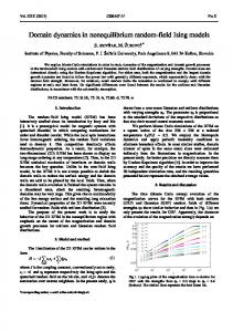
FIG. 1. 共Color online兲 Coordinates of the points studied by numerical simulations on the ␴-c diagram. The finite-size scaling analysis presented in Sec. IV is performed in regions I and II.

共4兲

where the sum extends over all the n . n. of Si. When a spin flips, it may trigger an avalanche. The unstable spins are flipped synchronously until a new stable situation is reached. The hysteresis loop is obtained by computing the magnetization N

m = 兺 Sici/N,

共5兲

i=1

as a function of the applied field H. Magnetization avalanches are recorded along the whole increasing field branch and their spanning properties are analyzed by using “mask” vectors 共as explained in Ref. 25兲 that allow them to be classified as nonspanning, 1D spanning, 2D spanning, and 3D spanning. In this work we shall mainly study the number of spanning avalanches of each kind which are recorded in the full upwards branch. These numbers, N1, N2, and N3, which depend on L, ␴, and c, correspond to averages over more than 104 realizations with different random fields and random vacancy positions. The disorder averages are denoted by the symbol 具·典. We study systems of sizes ranging from L = 8 to L = 64 at a number of points on the ␴-c diagram, as indicated schematically in Fig. 1.

where Si = ± 1 are Ising spin variables, ci = 0 , 1 indicates the presence of a vacancy 共ci = 0兲 or not 共ci = 1兲 at each site, hi are Gaussian-distributed quenched random fields with zero 3

冊

S jc j + hi + H ,

j

III. NUMERICAL RESULTS

The general evolution of the average hysteresis loops as a function of ␴ and c is shown in Fig. 2. One can observe the transition from discontinuous loops to smooth loops when ␴ or c are increased. It can also be seen that the saturation magnetization decreases with increasing c. Figure 3 shows the behavior of the coercive field 具Hcoe典 as a function of the concentration of vacancies for different values of ␴. As can be seen, 具Hcoe典 decreases with increasing c and increasing ␴. The behavior with increasing c exhibits an inflection point at the transition, as can be seen in the inset of Fig. 3, which shows the numerical derivative of the 具Hcoe典 with respect to c. Such an inflection point does not exist in the nondiluted model when the coercive field is plotted as a function of ␴. This feature, which can be of interest for the determination of the critical point in experiments, is probably related to the fact that 具Hcoe典, expressed as a function of c, should vanish at c ⱕ 1, whereas if it is expressed as a function of ␴ it only vanishes asymptotically when ␴ → ⬁. Figure 4 shows the distribution D共s ; ␴ , c , L兲 of avalanche sizes 共the size s of an avalanche is the number of spins

104409-2


DILUTED THREE-DIMENSIONAL RANDOM FIELD¼

FIG. 2. 共Color online兲 Average hysteresis loops corresponding to a system of size L = 32 for different values of ␴ and c as indicated.

flipped兲 for the same cases as in Fig. 2 on the log-log scale. The histograms include all avalanches irrespective of their spanning properties. The qualitative picture is that power-law distributions are obtained along a critical line with an expo4

< >/ ∂c ∂ Hcoe

-1.5

coe

3

-1

σ=0.5 σ=1.0 σ=1.5 σ=2.0

-2

-2.5 0

0.2

2

c

0.4

1 0

0.2

c

0.4

0.6

FIG. 3. 共Color online兲 The coercive field as a function of the vacancy concentration c for different values of the amount of disorder ␴. The inset shows the behavior of the numerical derivative ⳵Hcoe / ⳵c which exhibits a maximum at the transition line. Data correspond to averages in a system of size L = 64.

FIG. 4. 共Color online兲 Avalanche size distributions corresponding to a system with L = 32 at different values of c and ␴ as indicated. Data are represented on the log-log scale.

nent that seems to be the same for all values of c. Apparently, no differences can be observed when comparing the transition induced by changing ␴ from the transition induced by changing c. Below the critical line the distributions show a peak for large values of s which correspond to the 1D-, 2D-, and 3D-spanning avalanches. Above the critical line, the distributions have an exponentially damped character. Figure 5 shows the average number of 1D-, 2D-, and 3Dspanning avalanches as a function of ␴ for increasing values of the vacancy concentration c ranging from 0 to 0.5. Data correspond to a system with size L = 16. The same information is displayed in Fig. 6 for a system with size L = 48. The behavior for small and intermediate vacancy concentration is qualitatively similar to that found for the nondiluted model.25,27,28 The average numbers N1 and N2 display peaks, whereas N3 shows a peak on the edge of a step function. Note that for L = 16 the peak height in N1共␴ , c , L兲 and N2共␴ , c , L兲 seems to decrease with increasing c. This behavior, however, is much less apparent for larger systems 共L = 48兲. Therefore, it is possibly due to a finite-size effect. At higher concentrations 共c ⬎ 0.4兲 N1 and N2 begin to develop a flat plateau at low ␴. The reason for this plateau can be well understood by looking at the 3D plot in Fig. 7, which represents the average number N1共␴ , c , L兲 for L = 32. The plateau in the constant c cuts of Figs. 5 and 6 is due to the fact that the crest of the N1 and N2 functions does not decrease linearly with increasing c, but shows a bend and reaches the c axis almost perpendicularly.

104409-3



(a)

N1 (σ,c,L)

1 0.5

(b)

1 0.5 0 1.5

c=0.00 c=0.05 c=0.10 c=0.15 c=0.20 c=0.25 c=0.30 c=0.35 c=0.40 c=0.45 c=0.50

(c)

1 0.5 0 0

0.5

1

1.5

σ

2

2.5

3

L=48

0.5

(b)

1 0.5 0 1.5

(c)

c=0.00 c=0.05 c=0.10 c=0.15 c=0.20 c=0.25 c=0.30 c=0.35 c=0.40 c=0.45 c=0.50

1 0.5 0 0

3.5

FIG. 5. 共Color online兲 Average number of 共a兲 1D-spanning avalanches, 共b兲 2D-spanning avalanches, and 共c兲 3D-spanning avalanches, as a function of ␴ for different values of the vacancy concentration c, as indicated by the legend. Lines are guides to the eye. Data correspond to numerical simulations of a system with size L = 16.

(a)

1

0 1.5

N2 (σ,c,L)

N2 (σ,c,L)

0 1.5

N3 (σ,c,L)

1.5

L=16

N3 (σ,c,L)

N1 (σ,c,L)

1.5

0.5

1

1.5

σ

2

2.5

3

3.5

FIG. 6. 共Color online兲 Average number of 共a兲 1D-spanning avalanches, 共b兲 2D-spanning avalanches, and 共c兲 3D-spanning avalanches, as a function of ␴ for different values of the vacancy concentration c, as indicated by the legend. Lines are guides to the eye. Data correspond to numerical simulations of a system with size L = 48.

IV. FINITE-SIZE SCALING HYPOTHESIS

˜ 共uL1/␯兲, N␣共␴,c,L兲 = L␪N ␣

共6兲

where ␣ = 1 , 2 and u共␴ , c兲 is a scaling variable that measures the distance to the critical line. The exponents ␪ and ␯, as ˜ , were already found in previous well as the functions N ␣ 25 works. Therefore, the hypothesis is quite strong and indicates that all the N1 and N2 data, corresponding to different sizes L, different vacancy concentrations c, and different amounts of disorder ␴, must collapse onto a function that is already known. The only freedom that we have is in the determination of the scaling variable u that should be ana-

L=32 1.5 N1(σ,c,L)

The hypothesis that we want to check numerically is that in the presence of vacancies, the critical point found at c = 0 transforms into a critical line for a wide range of concentrations. Thus, the critical exponents found previously should be equally valid for the description of the behavior of the average numbers N1 and N2 with c ⬎ 0. According to this hypothesis we shall propose the following corresponding FSS behavior:

1 0.5 3 2.5

0 0

0.1 0.2 0.3 0.4 0 0.5 0.6 c 0.7

2 1.5 σ 1 0.5

FIG. 7. 共Color online兲 Surface plot representing N1共␴ , c , L兲 for L = 32. The dashed lines on the basal plane represent the position of the cuts in Fig. 8 at c = 0.15 and ␴ = 0.9.

104409-4



2

3

σ=0.9

(a)

2.5

L=16 L=32 L=48 L=64

1.5

σc = 2.21 +- 0.01 λ = -4.09 +- 0.03

2

σ

-θ ~ L N1(σ,c,L) / N1(0)

2.5

1.5

1 1

0.5 0.5

-θ ~ L N1(σ,c,L) / N1(0)

2.5

0.25

(b)

c

0.3

0.35

0 0

c=0.15

1.5 1

0.5 0

1

1.2

1.4

σ

1.6

1.8

FIG. 8. 共Color online兲 Examples of crossing points on the critical line along cuts 共a兲 parallel to the c axis and 共b兲 parallel to the ␴ axis. The different symbols correspond to different system sizes as indicated by the legend. Continuous lines are guides to the eye. The horizontal dashed line indicates the height 1 where the curves are supposed to cross according to Eq. 共7兲.

lytic. Before constructing it in the next section, we can make a first test of Eq. 共6兲 by checking scaling on the critical line. Note that by setting u = 0, Eq. 共6兲 becomes ␪˜

N␣共␴,c,L兲 = L N␣共0兲,

0.1

0.2

0.3

0.4

c

0.5

0.6

0.7

FIG. 9. 共Color online兲 Critical line in the ␴-c diagram determined from the crossing points in N1 共•兲 and N2 共⫻兲. The dashed line is the fit discussed in the text, and the thin discontinuous lines indicate the cuts along which the correlation in Fig. 14 is computed.

2

␴c共0兲 = 2.21 is in total agreement with the previous estimate for the nondiluted model.25 It is remarkable that the finite-size-scaling hypothesis allows the collapse of the data up to large values of c, far from the point c = 0, where the scaling function and the exponents were determined. It is also remarkable that scaling works even after the bend observed for c ⬎ 0.3. 关Note that the crossing point shown in Fig. 8共a兲 corresponds to a value of ␴ where the critical line is not linear.兴 For small values of ␴ the critical line displays vertical behavior. The critical value of the vacancy concentration cc above which the hysteresis loops do not display a discontinuity can be fitted to cc = 0.426± 0.003. V. SCALING VARIABLE

In general the scaling variable is a function that can be expanded as

1

共7兲

where ␴ and c should be on the critical line. Since we know ˜ 共0兲 = 0.12, and N ˜ 共0兲 = 0.07, 共from Ref. 25兲 that ␪ = 0.10, N 1 2 ˜ 共0兲 we can deduce that the different curves N␣共␴ , c , L兲 / L␪N ␣ should cross at height 1 on the critical line, independently of L. Two examples are shown in Fig. 8 that correspond to two cuts 共one at constant ␴ and the other at constant c兲 on the ␴c diagram. As can be seen, the critical line can be determined to high accuracy. By analyzing a large number of such ␴ and c cuts, we have managed to construct the critical line. The result is shown in Fig. 9. Note that the process can be repeated independently with N1 and N2. The two independent lines overlap almost perfectly. The obtained critical line is linear up to c ⯝ 0.3. A least-squares fit gives ␴c共c兲 = ␴c共0兲 + ␭c with ␴c共0兲 = 2.21± 0.01 and ␭ = −4.09± 0.03. The value

L=16 L=32 L=48 L=64

region I 0.8 ~ 1/ν N1(uL )

0 0.2

cp

0.6 0.4 0.2 0 -6

-4

-2

0

2

4

6

8

10

1/ν

uL

FIG. 10. 共Color online兲 Finite-size-scaling collapse of the average number of 1D-spanning avalanches in region I. The continuous line shows the Lorentzian function in Eq. 共12兲.

104409-5



1

L=16 L=32 L=48 L=64

region II 0.8 ~ 1/ν N2(uL )

0.8 ~ 1/ν N2(uL )

1

L=16 L=32 L=48 L=64

region I

0.6 0.4

0.6 0.4

0.2

0.2

0

0 -6

-4

-2

0

2

4

6

8

10

-6

-4

-2

1/ν

uL

0

2 uL

FIG. 11. 共Color online兲 Finite-size-scaling collapse of the average number of 2D-spanning avalanches in region I. The continuous line shows the Lorentzian function in Eq. 共13兲.

4

6

8

10

1/ν

FIG. 13. 共Color online兲 Finite-size scaling collapse of the average number of 2D-spanning avalanches in region II. The continuous line shows the Lorentzian function in Eq. 共13兲.

u共␴,c兲 = a0 + a1␴ + a2c + a3␴c + a4␴2 + a5c2 + ¯ . 共8兲

u共␴,c兲 = 共␴ − ␴c − ␭c兲共b0 + b1␴ + b2c兲.

ρε,b

(b) σ=0.5

0.3

0 0.6

(c) σ=0.1

ρε,b

~ 1/ν N1(uL )

0.8

0.3

0.6

L=16 L=32 L=48 L=64

region II

L=16 L=32 L=48 L=64

0

共9兲

We should also consider the fact that the scaling variable is known to be well described by a second-order expansion 共up to ␴2兲 for c = 0 as indicated in Eq. 共2兲. After some algebra

1

(a) σ=1.0 0.6

ρε,b

Since c and ␴ are not necessarily very small along the critical line, it is difficult to know a priori how many terms in the expansion will be needed in order to obtain a good scaling collapse. The direct determination of a large number of coefficients from the numerical data is difficult. Therefore, we shall adopt a different strategy by taking into account previously known data as much as possible. As a first step we will concentrate on the region c ⱕ 0.3 where the coexistence line shows linear behavior and we will try to use an expansion up to quadratic terms only. By forcing the condition u = 0 to be satisfied on the fitted coexistence line, we deduce that u satisfies

0.6

0.3

0.4 0.2

0 0

0 -6

-4

-2

0

2

4

6

8

10

1/ν

uL

FIG. 12. 共Color online兲 Finite-size scaling collapse of the average number of 1D-spanning avalanches in region II. The continuous line shows the Lorentzian function in Eq. 共12兲.

0.2

0.4

c

0.6

0.8

FIG. 14. 共Color online兲 Correlation between the border of the largest cluster of vacancies and the largest avalanche as a function of c. Data corresponding to different system sizes are represented by different symbols as indicated by the legend. The curves correspond to cuts in the phase diagram at 共a兲 ␴ = 1, 共b兲 ␴ = 0.5, and 共c兲 ␴ = 0.1.

104409-6



共14兲 coincide at ␴ = 0 and c = 0. Thus k⬘ = 共A − 1兲 / 共B − 1兲. The only free parameter for the collapse of the data is B. Best collapses are shown in Figs. 12 and 13 for N1 and N2, respectively, using the best choice B = −0.2 共thus k⬘ = 1兲. The continuous lines in both figures correspond to the same lines as in Figs. 10 and 11. We can thus conclude that we have built up two good approximations 关given by Eqs. 共9兲 and 共14兲兴 to the unique scaling variable in regions I and II which will display a more complex behavior in the intermediate region where the critical line bends, probably with higher order terms.

one can determine the two parameters b0 and b1, b0 = 共1 − A兲/␴c = 0.543 ± 0.002,

共10兲

共11兲 b1 = A/␴2c = − 0.041 ± 0.001. Therefore, we are left with a single free parameter b2 that should allow all of the data in the scaling region to collapse onto a single curve for different values of ␴, c, and L. All the available data in region I of Fig. 1 have been considered. Note also that the same b2 parameter must be used to scale both N1 and N2 data. The best two collapses are shown in Figs. 10 and 11 for b2 = −0.13. Note that the data for c = 0 are also included on this plot. Therefore, we have obtained two ˜ and N ˜ that are compatible with those of scaling functions N 1 2 Ref. 25. In this paper the scaling functions were approximated by Gaussians, although it was also shown that there were systematic deviations. In this work we have tried to fit the data using more complex functions 共with three free parameters兲. We have found a very good ␹2 by using the following modified Lorentzians, which are represented by a continuous line on the data in Figs. 10 and 11, ˜ 共x兲 = N 1

1 , 共1.73 − 0.53x + 0.10x2兲3.9

共12兲

˜ 共x兲 = N 2

1 . 共1.83 − 0.59x + 0.13x2兲4.6

共13兲

VI. DISCUSSION

In this section we will try to explain why the critical line exhibits such a curvature. There must be a physical reason that goes beyond the mere effect of the dilution of the system and destabilizes the phase even more with the ferromagneticlike discontinuity. We propose that the effect is related to the percolation of vacancies above c p = 0.3116, a value which is, indeed, very close to the limit where the critical line loses its linearity. To justify this hypothesis numerically, we have studied the distribution of the clusters of vacancies and the position of the avalanches for each particular realization of disorder. In particular, we have determined the spatial position of the largest vacancy cluster 共which, above c p, will correspond to the percolating cluster in the thermodynamic limit兲. It is clear that the neighboring sites of this percolating cluster of vacancies are an easy path for the propagation of an avalanche, since these sites have a smaller number of neighbors. To distinguish such sites we have defined a local flag that takes values bi = 1 when a site belongs to the border of the largest cluster of vacancies or bi = 0 otherwise. We have also recorded the largest avalanche during the H scan 共which will correspond to the spanning avalanche below the critical line in the thermodynamic limit兲 and we have marked its position with a flag ⑀i = 1. With these two variables we have defined the correlation between the border of the largest cluster of vacancies and the largest avalanche as

For a second step we will try to build up u共␴ , c兲 for the data very close to the ␴ = 0 axis. In this region II 共see Fig. 9兲 the transition line is again quite linear and, in fact, is almost vertical. This means that to measure the distance to the critical line it should be sufficient to use the variable 共c − cc兲. We have considered the following second-order expansion:

冉冊

c − cc u共c兲 c − cc = +B k⬘ cc cc

2

共14兲

.

Note that k⬘ is not a free parameter. It can be fixed by imposing that the definitions of the scaling variables 共9兲 and

␳⑀,b =

冓

冔冓兺冔冓兺冔冑冓兺冔冓兺冔冑冓兺冔冓兺冔 1 N

1 N

⑀2i

兺 ⑀ ib i −

−

1 N

⑀i

Note that since ⑀i and bi only take values of 1 and 0, the power 2 in the first bracket inside the square roots can be suppressed. This correlation is equal to 1 when the spanning avalanche sits exactly on the border of the spanning cluster of vacancies. The behavior of ␳⑀,b as a function of c is shown in Fig. 14 for three different values of ␴ that correspond to the dashed lines indicated in Fig. 9, and for increasing sys-

1 N 2

⑀i

1 N

1 N

b2i

bi

−

1 N

2

.

共15兲

bi

tem sizes as indicated by the legend. The important observation is that the curves for ␴ = 0.5 and ␴ = 0.1 exhibit two crossing points. One is located at c p and the other on the critical line 共it thus shifts with ␴兲. For a concentration of vacancies below c p or above the critical line, the behavior of the curves with increasing L indicates that the correlation vanishes in the thermodynamic limit, whereas in the region

104409-7



between the two crossing points the correlation increases with increasing system size. A value ␳ = 1 is probably not reached, since the spanning avalanche is larger than the border of the percolating cluster of vacancies. Using this analysis, we have thus identified the origin of the curvature of the critical line; when vacancies percolate, the spanning avalanche propagates along the border of the percolating cluster of vacancies. The propagation in such a constrained environment decreases the amount of disorder needed to break the infinite macroscopic avalanche into small microscopic jumps. However, as shown in Sec. V, this mechanism does not change the values of the critical exponents.

ties close to this line are characterized by the same critical exponents as in the nondiluted model. This result indicates that it should be possible to find RG arguments, showing that there is a unique fixed point at T = 0 in the disorder parameter space that includes, at least, both random fields and dilution.2 We have computed quadratic approximations to the scaling variable in two different zones of the phase diagram that allow for a bivariate finite-size-scaling collapse on a universal scaling function. Finally, we have proposed an explanation for the curvature observed in the critical line when the concentration of vacancies increases above the percolation limit; the spanning avalanche that is responsible for the discontinuity of the hysteresis loops has a tendency to follow the neighborhood of the percolating cluster of vacancies.

VII. SUMMARY AND CONCLUSIONS

We have analyzed the influence of dilution on the critical properties of the 3D-RFIM at T = 0 with metastable dynamics. We have shown that the critical point, associated with the change in the shape of the hysteresis loop from discontinuous to continuous loops, becomes a critical line which we have located on the ␴-c phase diagram. The critical proper-

*Electronic address: [email protected] †

Electronic address: [email protected] 1 J. P. Sethna, K. Dahmen, S. Kartha, J. A. Krumhansl, B. W. Roberts, and J. D. Shore, Phys. Rev. Lett. 70, 3347 共1993兲. 2 J. P. Sethna, K. Dahmen, and O. Perković, The Science of Hysteresis 共Elsevier Inc., New York, 2005兲, Vol. 2, Chap. 2, pp. 107–179. 3 J. Ortín, A. Planes, and L. Delaey, The Science of Hysteresis 共Elsevier Inc., New York, 2005兲, Vol. 3, Chap. 5, pp. 467–541. 4 F. Detcheverry, E. Kierlik, M. L. Rosinberg, and G. Tarjus, Phys. Rev. E 68, 061504 共2003兲. 5 B. Tadić, Eur. Phys. J. B 28, 81 共2002兲. 6 K. A. Dahmen and J. P. Sethna, Phys. Rev. Lett. 71, 3222 共1993兲. 7 K. A. Dahmen and J. P. Sethna, Phys. Rev. B 53, 14872 共1996兲. 8 D. Dhar, P. Shukla, and J. Sethna, J. Phys. A 30, 5259 共1997兲. 9 X. Illa, J. Ortín, and E. Vives, Phys. Rev. B 71, 184435 共2005兲. 10 X. Illa, P. Shukla, and E. Vives, Phys. Rev. B 73, 092414 共2006兲. 11 P. S. S. Sabhapandit and D. Dhar, J. Stat. Phys. 98, 103 共2000兲. 12 P. Shukla, Phys. Rev. E 63, 027102 共2001兲. 13 A. Berger, A. Inomata, J. S. Jiang, J. E. Pearson, and S. D. Bader, Phys. Rev. Lett. 85, 4176 共2000兲. 14 J. Marcos, E. Vives, L. Mañosa, M. Acet, E. Duman, M. Morin,

ACKNOWLEDGMENTS

We acknowledge fruitful discussions with M. L. Rosinberg, F. J. Pérez-Reche, and A. Planes. This work has received financial support from projects MAT2004-01291 共CICyT, Spain兲 and SGR-2001-00066 共Generalitat de Catalunya兲. X.I. acknowledges a grant from DGI-MEC 共Spain兲.

V. Novák, and A. Planes, Phys. Rev. B 67, 224406 共2003兲. K. L. Babcock and R. M. Westervelt, Phys. Rev. Lett. 64, 2168 共1990兲. 16 P. J. Cote and L. V. Meisel, Phys. Rev. Lett. 67, 1334 共1991兲. 17 E. Vives and A. Planes, Phys. Rev. B 50, 3839 共1994兲. 18 W. Wu and P. W. Adams, Phys. Rev. Lett. 74, 610 共1995兲. 19 Ll. Carrillo, Ll. Mañosa, J. Ortín, A. Planes, and E. Vives, Phys. Rev. Lett. 81, 1889 共1998兲. 20 E. Puppin, Phys. Rev. Lett. 84, 5415 共2000兲. 21 G. Durin and S. Zapperi, Phys. Rev. Lett. 84, 4705 共2000兲. 22 M. P. Lilly, P. T. Finley, and R. B. Hallock, Phys. Rev. Lett. 71, 4186 共1993兲. 23 B. Tadić, Phys. Rev. Lett. 77, 3843 共1996兲. 24 M. C. Kuntz, O. Perković, K. A. Dahmen, B. Roberts, and J. P. Sethna, Comput. Sci. Eng. 1, 73 共1999兲. 25 F. J. Pérez-Reche and E. Vives, Phys. Rev. B 67, 134421 共2003兲. 26 F. J. Pérez-Reche and E. Vives, Phys. Rev. B 70, 214422 共2004兲. 27 O. Perković, K. A. Dahmen, and J. P. Sethna, cond-mat/9609072 共unpublished兲. 28 For a discussion of the problems in the nondiluted 2D RFIM, see Ref. 27. 15

104409-8