Oct 8, 1999 - We present an exact solution of the 1-D Random Field Ising Model (RFIM) ..... point, alignment to random elds only), a ferromagnetic phase for ...
Random Field Ising Chains with Synchronous Dynamics N.S. Skantzos
A.C.C. Coolen
Department of Mathematics, King's College London Strand, London WC2R 2LS, U.K. October 8, 1999
Abstract
We present an exact solution of the 1-D Random Field Ising Model (RFIM) with synchronous rather than sequential spin-dynamics, whose equilibrium state is characterised by a temperature-dependent pseudo-Hamiltonian, based upon a suitable adaptation of the techniques originally developed for the sequential (Glauber) dynamics RFIM. Although deriving the solution is somewhat more involved in the present model than in the case of the sequential RFIM, we are able to prove rigorously that the physics of the two RFIM versions are asymptotically identical. We thus recover the familiar Devil's Staircase form for the integrated density of local magnetisations, and nd a non-zero ground state entropy with an in nite number of singularities as function of the random eld strength.
Contents
1 Introduction 2 Model De nitions 3 Simple Solvable Detours
3.1 In nite Range Version of the Model . . . . . . . . . . . . . . . . . . . . . . . . . 3.2 Short-Range Interactions and Non-Random Fields . . . . . . . . . . . . . . . . .
2 3 5 5 9
4 Solution for Short-Range Interactions and Random Fields
11
5 Physical Properties of the Model
17
6 Discussion
22
4.1 Adaptation of the RFIM Techniques . . . . . . . . . . . . . . . . . . . . . . . . . 11 4.2 Statistics of Local Observables . . . . . . . . . . . . . . . . . . . . . . . . . . . . 14 4.3 Link Between Synchronous and Sequential Dynamics . . . . . . . . . . . . . . . . 15
5.1 The Devil's Staircase and the Free Energy . . . . . . . . . . . . . . . . . . . . . . 17 5.2 Entropy and Ground State Degeneracy . . . . . . . . . . . . . . . . . . . . . . . . 21
1
1 Introduction The one-dimensional random eld Ising model is one of the most extensively studied disordered systems [1, 2, 3, 4, 5, 6, 7, 8, 9, 10]. Most of the exact solutions that have been presented rely on a method which goes back to [1]: conditioning the partition function ZN of an N -spin chain on the state �N of the last spin (giving the two quantities ZN;�1 ), and subsequently constructing a recurrence relation expressing the ZN +1;�1 in terms of the ZN;�1 . The free energy of the system can be written as an integral over the distribution of the subsequent ratios kN of the conditioned partition functions ZN;�1 . Adding new spins to the chain one by one (and thus also new random elds) de nes a discrete markovian process for these ratios, or their probability density PN (k), whose stationary state P1 (k) fully determines the asymptotic free energy per spin. In early papers based on this technique, approximations of the stationary solution were calculated in certain parameter regimes, e.g. for zero temperature [2]. It was later shown [3] that Rin certain regions of parameter space, including T > 0, the integrated stationary density P^ (k) = 0k dz P (z ) acquires the form of a highly non-analytic object known as the Devil's Staircase. The support of the density P (k) is now known to be a zero-measure Cantor set [8, 9, 11], and the spectrum f (�) of generalised dimensions has been fully calculated [12, 13]. Phase transitions in the usual thermodynamic sense are absent, but the transition of the fractal dimension of the support of P (k) to DF < 1 has signi cant physical consequences; in particular, there are regions in the phase diagram where observables such as the local magnetization take values only from a disconnected set. In this paper we study an alternative to the more standard types of 1-dimensional RFIM models. Here the stochastic microscopic alignment of spins to local elds is not executed sequentially (according to a Glauber rule, leading to the conventional Boltzmann-type equilibrium distribution with the standard Ising Hamiltonian), but the spin states are updated synchronously, i.e. in parallel, at discrete time-steps. Ising models with synchronous dynamics have been studied e.g. in the context of neural networks [14, 15] and probabilistic cellular automata (see e.g. [16]). Synchronous execution of the (originally sequential) Glauber laws is known to lead again to a unique equilibrium state [15], which can formally be written in the Boltzmann form, and which in principle enables equilibrium statistical mechanical calculations. However, the parallel dynamics (pseudo) Hamiltonian is a function of temperature, and thermodynamic relations will generally have to be modi ed. What is known about the relation between the equilibrium physics of the two types of dynamics concerns mostly in nite-range models. To be speci c: in the case of predominantly negative exchange interactions the two dynamics types clearly lead to completely di�erent physics, with period-two limit-cycles appearing in the synchronous dynamics case. In the case of predominantly positive exchange interactions, however, the picture is less clear. For instance, the phase diagram of the Sherrington-Kirkpatrick [17] model (with J0 � 0) appears not to be a�ected by synchronous dynamics [18], whereas for the Hop eld model [19] the phase diagram does change [20]. We are not aware of equilibrium studies involving disordered spin chains with synchronous dynamics. Before solving the short-range parallel dynamics RFIM we rst prepare the stage by making two relatively simple (but also as yet unsolved) instructive detours: we solve both statics and dynamics of the in nite-range version of the model, and we solve the parallel dynamics Ising chain (without random elds) in equilibrium. In solving the parallel dynamics RFIM we nd that the standard RFIM techniques need to be adapted, in that conditioning of the partition function on the state of the last spin in the chain is no longer su�cient. The present model involves a more 2
complicated stochastic process in terms of three ratios of conditioned partition functions rather than one. We then solve the model, and show that asymptotically the expectation values of the local magnetisations of sequential and parallel dynamics become identical. We examine the occurrence and properties of the Devil's Staircase shapes for the integrated probability densities of the relevant observables, and we calculate the ground state entropy, which exhibits the nontrivial behaviour as a function of the random eld strength which had also been observed for sequential dynamics chains [5].
2 Model De nitions
Our model is de ned as a collection of N Ising spins � = (�1 ; : : : ; �N ) 2 f?1; 1gN , arranged in a one-dimensional chain. The dynamics is a stochastic alignment to local elds of the familiar form, however, in contrast to the more conventional Glauber-type rules where individual spin updates are made sequentially, here the individual spin updates are made in a fully synchronous way at each discrete time step: (1) 8i 2 f1; : : : ; N g : Prob[�i (t + 1)= �1] = 21 [1 � tanh[ hi (� (t))]]
hi(�(t)) =
N X
j =1
Jij �j (t) + �i
(2)
The parameter = 1=T controls the amount of stochasticity in the dynamics; for = 1 the process (1) is a deterministic map, for = 0 is a fully random map. The variables Jij and �i represent spin interactions and external elds, respectively. The Markov chain (1) can alternatively be de ned in terms of the microscopic state probability pt (� ):
pt+1 (�) =
X
�0
W [�; � 0 ] pt (� 0 )
W [�; � 0] =
N Y e �i hi �0 (
)
i=1 2 cosh[ hi (� )]
0
(3)
For any nite and nite N the process (3) is ergodic and evolves into a unique stationary distribution p1(� ). It can be shown that this is an equilibrium state (obeying detailed balance) if and only if Jij = Jji for all pairs (i; j ). In particular, there is no need to exclude selfinteractions, which would have been required to nd detailed balance in models with sequential dynamics. In the detailed balance case the corresponding equilibrium state probabilities can only formally be written in the Boltzmann form p1 (� ) � exp[? H (� )], with the so-called pseudo-Hamiltonian 1 H (� ), which was rst derived in [15]:
H (� ) = ? 1
N X i=1
log[2 cosh( hi (� ))] ?
N X i=1
�i �i
(4)
Due to the synchronous execution of the alignment dynamics, and the resulting non-Gibbsian equilibrium distribution, conventional thermodynamic relations will generally no longer hold. We can still formally de ne a free energy per spin as X (5) f = ? 1 log e? H (�) N
N
�
1 Note that this pseudo-Hamiltonian depends on , hence the name.
3
which will play a useful role as a generating function for equilibrium averages, but which no longer carries the usual thermodynamic signi cance. In this study we consider the case where the external elds �i have been drawn independently at random from a symmetric binary distribution w(�) with variance �~2 , and we choose spin interactions Jij describing a strictly ferromagnetic (J > 0) or strictly anti-ferromagnetic (J < 0) (periodic or open) 1-D chain: Jij = J (�j;i+1 + �j;i?1 ) (6) w(�) = 21 �[� ? �~] + 21 �[� + �~] R We can always put �~ � 0. Averages over w(�) will be denoted as: g(�) = d� g(�)w(�). The relevant macroscopic equilibrium observables in this system are the overall magnetisation m, the overall alignment u to the random elds and the next-time/nearest-neighbour correlation function a: X X m = lim 1 h� i u = �~?1 lim 1 � h� i (7) N !1 N i
i
N !1 N i
eq
1 a = Nlim !1 N
X i
h�i tanh[ hi (� )]i +1
i
i
eq
(8)
eq
in which the equilibrium averages are calculated using the Boltzmann distribution with the pseudo-Hamiltonian (4). Note that m; a; u 2 [?1; 1]. The order parameter a measures equilibrium state correlations of nearest neighbour spins probed at di�erent but successive times, which follows from the identity Z� h� tanh[ h (�)]i = lim 1 dt � (t)� (t + 1) i
i+1
eq
� !1 �
0
i
i+1
The observables m and u follow as moments of the joint distribution for random elds and local equilibrium magnetisations: X P � (�) = lim 1 � �[� ? h� i ] (9)
R
N !1 N i �i ;��~
i
eq
R
since m = d� �[P + (�) + P ? (�)] and u = d� �[P + (�) ? P ? (�)]. Using simple general properties such as h�i ieq = htanh[ hi (� )]ieq , which follows directly from stationarity of (3), we also see that (5) generates @f (10) a = ? 12 @J u = ? 21 @~fN N
@�
In order to identify the physical mechanisms responsible for the properties of the phase diagrams which we will nd in a subsequent section we now rst turn to the in nite range (strictly mean eld) version of the present model with synchronous dynamics and random elds. In addition this will aid our interpretation and characterization of the various phases in our phase diagrams. 4
3 Simple Solvable Detours The three key ingredients which in combination render the present model non-trivial are (i) the short-range connectivity, (ii) the random external elds, and (iii) the synchronous dynamics leading to a non-Boltzmann equilibrium state. If we replace the synchronous dynamics by a standard sequential Glauber one we recover the standard random eld Ising model [2, 3], exhibiting transitions to non-trivial states where the integrated distribution of local magnetizations acquires the form of a Devil's Staircase and where h�i ieq itself takes values from the Cantor set [4]. In this section we work out the simple solvable models obtained upon either sacri cing the short-range connectivity (retaining random elds and synchronous dynamics) or sacri cing the random elds (retaining short-range interactions and synchronous dynamics).
3.1 In nite Range Version of the Model
As usual, the in nite range version of the present model is obtained upon replacing the nearest neighbour interactions Jij = J [�i;j +1 + �i;j ?1 ] by suitably re-scaled uniform ones, viz. Jij = J=N . Solving this model rst allows us to disentangle the e�ects of random elds and synchronous dynamics from those generated by the short-range nature of the interactions. We calculate combining (4) with (5),Pand by inserting the exR the free energy per spin bypartition pression 1 = dm �[m ? m(� )] into the function Z = � exp[? H (� )], where P ? 1 ~ m = (m; u; a) and where m(�) = N i �i(1; �i =�; tanh[ hi+1 (�)]). This makes sure that our calculation is formulated in terms of the order parameters of interest. We then replace the delta functions by their integral representations and perform the spin summations, leading to: Z 1 ^ ) ^ e? N�N (m;m log dmdm (11) f = ? lim 1
where
N !1 N
1 ^ ) = ?im � m ^ ? u�~ ? N �N (m; m 1 ? N
X i
X i
log[2 cosh[ (Jm + �i )]]?
log[2 cosh[ (im^ + ia^ tanh[ (Jm + �i+1 )] + iu^�~?1 �i)]]
^ ) is for N ! 1 evaluated by gradient descent, whereby the free energy The integral over (m; m ^ ) evaluated at the physical saddle point. Di�erentiaper spin follows as the exponent �1 (m; m ^ ) with respect to m and m ^ leads us to the following three coupled non-linear tion of �1 (m; m equations: m = GJ (GJ (m)) u = �~?1 � tanh[ (JGJ (m) + �)] a = m GJ (m) (12) in which GJ (m) = tanh[ (Jm + �)] d GJ (m) > 0 The function GJ (m) is anti-symmetric due to w(�) = w(?�), and monotonic, with dm d for J > 0 and dm GJ (m) < 0 for J < 0. We do not consider the trivial case J = 0. The saddlepoint problem is autonomous in m, with u and a simply following as slave variables. It is easily demonstrated that the equations (12) are solved by the solution of the following (simpler) ones: m = GjJ j(m) u = �~?1 � tanh[ (jJ jm + �)] a = m2 sgn(J ) (13) 5
It is in fact the unique solution. This follows from a simple argument, which relies only on the two d G (m) > 0 and GJ (GJ (m)) = G (G (m)). All solutions of the saddle-point properties dm jJ j jJ j jJ j equations (12) obey:
h
i
h
ih
h
ih
0 � m ? GjJ j(m) = m ? GjJ j(m) GJ (GJ (m)) ? GjJ j(m) 2
i
i
= m ? GjJ j(m) GjJ j(GjJ j(m)) ? GjJ j(m) � 0 Thus we always have m = GjJ j(m). Using (13) and the identity GJ (m) = sgn(J )GjJ j (m) we then obtain for the value of the asymptotic free energy per spin (11) the following expression: (14) f = m2 jJ j ? 2 log 2 ? 2 log cosh[ (jJ jm + �)] 1
Note that this is precisely twice the free energy that would have been found for sequential Glauber-type mean- eld systems. Due to the fact that the uctuations in the global magnetisation m vanish for N ! 1, we can also conclude, using h�i ieq = htanh[ hi (� )]ieq = tanh[ (Jm + �i )], that the distribution de ned in (9) reduces simply to a delta peak: h i (15) P � (�) = 12 � � ? tanh[ (Jm � �~)] A bifurcation analysis of equation (13) will allow us to determine the dependence of the key order parameter m on the system parameters J and �~, and lead to a phase diagram. For our present choice (6) of random eld distribution both continuous and discontinuous bifurcations of non-zero solutions of m = GjJ j(m) are found to occur, away from the trivial solution m = 0 (which is always present). The continuous transition lines can be determined in explicit form in the (�~; J ) plane, the discontinuous ones can be calculated in the form of parameterizations f�~(x); J (x)g, with x = 2 Jm 2 < and with f�~(?x); J (?x)g = f�~(x); J (x)g: continuous bifurc: : J = � cosh2 ( �~) (16) h x) cosh(x)?x i 2 1 x tanh(x) ; J ( x ) = � discontinuous bifurc: : �~(x) = 21 acosh xsinh( 2 x?tanh(x) cosh(x)?sinh(x) These results can easily be veri ed by insertion into the two bifurcation conditions m = GjJ j(m) d G (m). The resulting phase diagram is drawn in gure 1. The symmetry of and 1 = dm jJ j the phase diagram with respect to J ! ?J follows immediately from the invariance of (13) under this transformation. The two discontinuous lines start at the branching points p transition 3 1 ? ? ~ ~ ( � ; J ) = limx!0 ( �(x); J (x)) = ( 2 log[2 + 3]; � 2 ), where each connects to a continuous transition line. The characterization of the observed phases in gure 1 is greatly simpli ed by the dynamical solution of the long-range model, which we describe next. The in nite range version of our model is su�ciently simple to also allow for an exact dynamicalPsolution. Here we analyse the evolution of the observables m(� ) = (m(� ); u(� ); a(� )) = 1 ~ N i �i (1; �i =�; tanh[ hi+1 (� )]), whose macroscopic probability density Pt (m) evolves according to Z Pt+1 (m) = dm0 Wt [m0 ! m] Pt (m0) (17) 6
with the macroscopic transition densities P 0 �[m ? m(�)]�[m0 ? m(�0)] p (�0 ) W [�; �0] 0 P 0 �[m0 ? m(�0 )] p (�t0) Wt [m ! m] = �� t � In this expression we insert equations (1) and (3). Since the local elds depend on the microscopic state � only through the functions m(� ) the microscopic distribution pt (� 0 ) drops out of the transition density Wt [: : :] which thereby loses its explicit time-dependence:
� W [m0 ! m] = e N Jmm0
1 �u? N
+~
P
�X
0
i log 2 cosh[ (Jm +�i )]
�
�[m ? m(�)]
Upon replacing the delta function by its integral representation and performing the spin summations we then arrive at
� �Z ^ e? N�N m;m0 ;m W [m0 ! m] = N d m 2� 3
where
^ )
(
^ ) = ?im ^ � m ? Jmm0 ? �~u + 1 �N (m; m0 ; m N
X i
log 2 cosh[ (Jm0 + �i )]
1 X log 2 cosh[ (im^ + ia^ tanh[ (Jm + � )] + iu^� �~? )] ? N i i +1
i
1
In the limit N ! 1 the macroscopic transition density is seen to be dominated by the phys^ ) (for xed m0 ). Di�erentiation with respect to m and m ^ ical saddle-point of �1 (m; m0 ; m immediately leads us to
13 2 0 3 20 1 0 tanh[ (Jm0 + �)] m ! m m 6 u C ? BB CC77 lim W 64 u0 ! u 75 = � 64B �~? � tanh[ (Jm0 + �)] @ A @ A5 N !1 a0 ! a a tanh[ (Jm + �)] tanh[ (Jm0 + �)] 1
For N ! 1 the macroscopic observables (m; u; a) apparently evolve deterministically according to the following coupled non-linear maps: ut+1 = �~?1 � tanh[ (Jmt + �)] (18) mt+1 = tanh[ (Jmt + �)]
at+1 = tanh[ (Jmt+1 + �)] tanh[ (Jmt + �)]
(19)
Although the xed-points of the maps (18,19) are identical to those that would have been found for a similar system but with sequential Glauber dynamics, the stability properties of such xed-points can be quite di�erent. In particular, for J < 0 and low temperatures (where a sequential system would evolve towards the m = 0 state) the present system, endowed with fully synchronous dynamics, evolves into a stable macroscopic period-2 limit-cycle of the form at = ?(m? )2 mt = (?1)t m? ; ut = �~?1 � tanh[ (Jm? + �)]; with
m? = tanh[ (jJ jm? + �)] 7
1.0
4
m=0
xed-point 0.5
3
�~
both
both
m
2
1
m 6= 0
0
−8
−4
−0.5
m 6= 0
2-cycles
0.0
xed-points 0
4
−1.0 0.0
8
0.5
1.0
1.5
2.0
�~
J
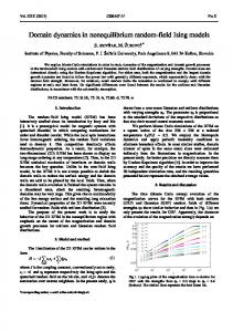
Figure 1: Left: phase diagram of the in nite range version of the random eld Ising model with synchronous dynamics. We nd a paramagnetic phase around J = 0 (m = 0 xedpoint, alignment to random elds only), a ferromagnetic phase for large positive J (two m 6= 0 xed points), and a phase for large negative J exhibiting stable 2-cycles with oscillating magnetisation. In addition we have two intermediate regions (the rst between the paramagnetic and the ferromagnetic region, and the second between the paramagnetic and the 2-cycle region) where both the m = 0 state and the m 6= 0 states are locally stable; here the nal state is dictated by initial conditions. Dashed lines indicate p rst order transitions, solid lines indicate second order ones; the two touch when �~ = 12 log[2 + 3], J = � 23 . Right: bifurcation diagram, showing the solutions m of the saddle-point equation as a function of �~ for J 2 f1 21 ; 2; 2 12 ; 3; 3 21 g (from left to right). This illustrates the appearance of discontinuous bifurcations and multiple locally stable solutions for J > 23 . In gure 1 we present the results of our analysis of the in nite range version of our model, in terms of phase- and bifurcation-diagrams. We have found (i) a paramagnetic region in parameter space where m = 0 only, (ii) regions where both the m = 0 state and m 6= 0 states are locally stable (both giving local minima of the free energy per spin), and (iii) regions where only m 6= 0 states are locally stable. The transitions (i) ! (iii) and (ii) ! (iii) are continuous, whereas (i) ! (ii) is discontinuous; the transition lines are given by (16). In the paramagnetic region the only tendency of the spins is to align to the random elds, with a constant non-zero value for u. On the other hand, in those regions where m 6= 0 xed points are locally stable, the combination of our statical and dynamical analysis leads to the conclusion that for J > 0 the m 6= 0 states represent ferromagnetic macroscopic xed points, whereas for J < 0 the system will evolve into a stable macroscopic 2-cycle, with only the absolute values of m and u being stable, but with the signs continually alternating in time. The latter phenomenon, anti-ferromagnetic exchange interactions inducing stable period-2 oscillations rather than an anti-ferromagnetic state, is typical for systems with synchronous 8
dynamics [20]. It implies that we have to be more careful in dealing with ergodicity breaking phenomena than when dealing with conventional systems. In the present model we nd ergodic components with m > 0 as well as their mirror images with m < 0, for su�ciently low temperatures. However, for J < 0 the relation between ensemble averages and time-averages is more subtle than usual. Only if we probe strictly at even time steps (or strictly at odd time steps) are we allowed to treat the system as if trapped in one ergodic component; if we do not distinguish between even and odd times and calculate temporal averages in the standard manner, all expectation values must be averaged over the values they take in each of the equivalent ergodic components, such that e.g. (15) must be replaced by h i h i (20) P � (�) = 21 � � ? tanh[ (Jm � �~)] + 12 � � ? tanh[ (?Jm � �~)]
3.2 Short-Range Interactions and Non-Random Fields
In the spirit of the previous sub-section we now inspect separately the e�ect of operating the spin alignments synchronously in a 1-D spin chain (with nearest neighbour interactions), with as yet uniform rather than random external elds �i = �. This in order to rst see in the simpler non-random case how the transfer matrix formalism is to bePadapted to accommodate the pseudo-Hamiltonian (4). We de ne a partition function ZN = � e H (� ) and calculate the free energy per spin (5). We then immediately nd
ZN =
N h XY
�i
=1
2 cosh [J (�i?1 + �i+1 )+ �] e �
N P �i i X Y i
=
�i
=1
T�syn i?1 �i+1
with the synchronous dynamics transfer matrix T�syn�0 = 2 cosh [J (� + �0 )+ �] e 21 �(�+�0 ) , or � (2J+�)] cosh[ �] T syn = 2 e cosh[ cosh[ �] e? � cosh[ (2J?�)]
!
(21)
We notice that, unlike the conventional transfer matrix for sequential Glauber-type processes, here the elements T�syn i?1 �i+1 couple spins which are next-nearest neighbours in the chain, and the corresponding matrix multiplications produce di�erent outcomes for even versus odd chainlengths: periodic boundaries :
N even : N odd :
n o ZN = Trace [T N= ] ZN = Trace [T N ] 2 syn
2
(22)
syn
In the case of open boundaries the results are, as always, slightly more messy. Here one nds, after some bookkeeping of boundary terms: open boundaries :
N even : N odd :
ZN = hajT N= ? = jbi ZN = hajT N= ? = jai hbjT N= ? = jbi 2 syn
1 2
2 syn
1 2
2
2 syn
3 2
in which
jai = (e 12 � ; e? 12 � )
jbi = 2(e 12 � cosh [J + �]; e? 21 � cosh [J ? �]) 9
(23)
From (22) and (23) we recover a result familiar from ordinary Boltzmann-type equilibrium systems, that in the thermodynamic limit for both types of boundaries the free energy per spin is expressed in terms of the largest eigenvalue �+ of the transfer matrix (21): f = ? lim 1 log Z = ? 1 log � 1
N
N !1 N
+
(with more prominent nite size e�ects in the case of open boundaries). The eigenvalues of (21) are found to be �2 � q 2 2 J ? 4 J �� = e cosh[ �] � sinh [ �] + e so that
� � q 2 2 ? 4 J f1 = ?2J ? log cosh[ �] + sinh [ �] + e
(24)
This is exactly twice the free energy per spin one would have found in the case where the dynamics in this system had been executed sequentially according to a Glauber rule (with an equilibrium distribution of the Boltzmann form). The magnetisation m and the next-time nearest-neighbour correlation function a follow directly upon using the free energy (24) as a generating function, in combination with the identity htanh[ hi (� )]i = h�i i: 1 Xh� i = ? 1 @ f = q sinh[ �] m = Nlim (25) !1 N i i eq 2 @� 1 sinh2 [ �] + e?4 J 1 Xh� tanh[ h (� )]i = ? 1 @ f a = Nlim i+1 eq !1 N i i 2 @J 1
q cosh[ �] sinh [ �] + e? J + sinh [ �] ? e? J q = ? J ? J 2
2
4
cosh[ �] sinh2 [ �] + e
4
+ sinh2 [ �] + e
4
(26)
4
which, again, is what would also have followed from sequential Glauber dynamics. Finally, to clarify the relation between the free energies obtained for sequential and synchronous dynamics it is advantageous to also carry out the above calculation in an alternative Q way, by rewriting the term i 2 cosh[ hi (� )] as a sum over an auxiliary set of Ising spin variables � = (�1; : : : ; �N ) leading to:
ZN =
XX
� �
1 P [�i Jij �j +�i Jij �j ]+ � P [�i +�i ] 2 i e ij
For periodic boundary conditions one then nds that
ZN =
N h XX Y
� �
i=1
i n
T�i �i+1 :T�i �i+1 = seq
seq
Trace [T N
seq
]
o
2
(J +�) ? J T seq = ee? J e e(J ?�)
!
where T seq is precisely the conventional (sequential dynamics) transfer matrix. The link with our previous results is now established by observing the identity T syn = T 2seq , which directly explains why the synchronous dynamics free energy (24) is twice the sequential dynamics one. 10
4 Solution for Short-Range Interactions and Random Fields We now return to the full model (2,3,6), with short-range spin interactions (and open boundary conditions), with random external elds �i 2 f?�~; �~g (drawn independently, with equal probabilities) and with synchronous dynamics. We solve this model using a suitable adaptation of the techniques in [2, 3], i.e. by studying the e�ect on the partition function ZN of adding one extra spin to the chain (and thus one extra random eld), which can be described by a Markovian stochastic map for a nite number of characteristic quantities. In the present model with synchronous dynamics, however, this map is considerably more complicated than that found in [2, 3]. Due to the repeated occurrence of terms of the form cosh [J (�i?1+�i+1 )+�i ] in the synchronous dynamics partition function, adding one spin induces e�ects which propagate backward over two sites, rather than just one; thus, in order to ensure a closed Markovian form for the map to be created we need to keep track of the states of the last two spins in the chain.
4.1 Adaptation of the RFIM Techniques
In order to nd the free energy P per spin (5) we have to calculate the synchronous dynamics partition function ZN = � e H (� ) , with the pseudo-Hamiltonian (4), which for an open chain reads
ZN =
X
�1 :::�N
1 [0; �1 ; �2 ]
"NY?
1
i=2
#
i [�i?1 ; �i ; �i+1 ] N [�N ?1 ; �N ; 0]
(27)
where
i [�i?1 ; �i ; �i+1 ] = 2 cosh [J (�i?1+�i+1 )+�i ] e �i �i We adapt the construction in [2, 3] and write for N > 1 the partition function (27) as the sum of four new quantities, which can be interpreted as conditional partition functions in which the states of the last two spins in the chain are prescribed:
ZN = ZN;"" + ZN;"# + ZN;#" + ZN;##
(28)
For N > 2 they are given by
0 0 1 1 ZN;"" � � � ; � ; N ? 1 N # " NY ? B BB ��N ?1 ; ��N;? CC X ZN;"# C B C
[ � ; � ; � ]
[ � ; � ; 0] =
[0 ; � ; � ] B B@ �� ;? �� ; CA (29) C i i ? i i N N ? N @ ZN;#" A �1:::�N N ?1 N i ��N ?1 ;? ��N;? ZN;## For N = 2 one simply has Z ;?? = [0; ?; ?] [?; ?; 0], for all (??) 2 f(""); ("#); (#"); (##)g. For 1
1
1
1
1
2
+1
1
=2
1
1
1
1
1
2
1
1
1
2
future use we also mention the following simple identity Z2;"#Z2;#" = 1[0; 1;?1] 1 [0;?1; 1] 2[1;?1; 0] 2 [?1; 1; 0] = 1 Z2;""Z2;## 1[0; 1; 1] 1 [0;?1;?1] 2[1; 1; 0] 2 [0;?1;?1]
(30)
which immediately follows from the above de nition of the functions i [: : :]. Enlarging the chain from N to N+1 spins gives rise to four new conditional partition functions fZN +1;?? g, which can be expressed in terms of the previous fZN;?? g. Note that, in contrast to the situation with the standard random eld Ising chains [2, 3], here this would not have been 11
possible if we had only conditioned the partition function on the state of the last spin �N of the chain, i.e. the fZN +1;? g cannot be expressed in terms of the fZN;? g. After some simple bookkeeping we can derive from (29) the following recurrent relations:
ZN ZN
;"" ;"#
+1 +1
!
= M + [�N +1
; �N ] ZZN;"" N;#"
!
ZN ZN
;#" ;##
+1 +1
!
= M ? [�N +1
in which the two (random) matrices M � [�N +1 ; �N ] are de ned via
0 �0 e M �[�0; �] = 2 cosh[ (�0 � J )] @ 0
10
(�+2J )] 0 A @ cosh[ cosh[ (� +J )] 0 cosh[ � ]
e? �
� J
cosh[ ( + )]
; �N ] ZZN;"# N;##
�] �?J )] cosh[ (� ?2J )] cosh[ (� ?J )] cosh[ cosh[ (
1 A
!
(31)
(32)
These then combine to form a four dimensional stochastic process, generated by 4 � 4 random matrices M [�N +1 ; �N ], the stationary state of which will lead us to the free energy per spin: 0 M + [�0; �] 0 M12+ [�0; �] 0 1 11 C B + 0 + 0 (33) M [�0; �] = BBB M210[� ; �] M ? 0[�0; �] M220[� ; �] M ? 0[�0; �] CCC A @ 11 12 0 M21? [�0; �] 0 M22? [�0; �]
80 1 0 19 > > Z [ � ; � ] 1 ; "" # " > BB Z ;"# [� ; � ] CC> > !1 N ;#" > :@ 11 A i ; Z [� ; � ] > 1
+1
=2
2
2
1
2
2
1
2
2
1
2
1
;##
2
(34)
In order to evaluate (34) it will turn out helpful to de ne the following three ratios of the conditional partition functions: (�n+J )] Zn;## (3) 2 �n Zn;## kn(2) = cosh[ k = e (35) kn(1) = e2 �n ZZn;"# n cosh[ (�n?J )] Zn;"# Zn;#" n;"" From the recurrent relations (31) it follows that the ratios (35) are successively generated by (3) (1) (2) (�n?2J )] kn(1)+1 = kn(3) cosh[ �n ] + kn kn (1)cosh[ (2) kn cosh[ (�n+2J )] + kn kn cosh[ �n ] (2) (�n?2J )] kn(2)+1 = e?2 �n kn(1) kn(3) (3) cosh[ �n ] + kn(1) cosh[ (2) kn cosh[ �n ] + kn kn cosh[ (�n?2J )] (2) (�n?2J )] kn(3)+1 = cosh[ �n] + kn cosh[ (2) cosh[ (�n+2J )] + kn cosh[ �n ] We note from these iterative equations that if kn(1) = kn(3) , then also kn(1)+1 = kn(3)+1 . Furthermore, it follows from identity (30) that k2(1) = k2(3) . Thus we are guaranteed that kn(1) = kn(3) for all n � 2, which simpli es our equations considerably: ~] + kn(2) cosh[ (�n?2J )] cosh[ � (1) (3) (1) (2) ?2 �n k(1) kn+1 = k k n n +1 = kn+1 n +1 = e (2) cosh[ (�n+2J )] + kn cosh[ �~]
12
Further substitution of the second of the above equations into the rst leads us to a markovian stochastic process for just a single random variable kn � kn(1) : ~] + e?2 �0 k0 cosh[ (�?2J )] cosh[ � 0 0 kn+2 = [kn ; �n+1 ; �n] [k ; �; � ] = (36) cosh[ (�+2J )] + e?2 �0 k0 cosh[ �~] In terms of probability densities, the stochastic process (36) can equivalently be written as XZ 0 � � Pi+2 (k) = 41 dk � k ? [k0 ; �; �0 ] Pi (k0 ) (37) �;�0 Following in the footsteps of [2, 3] we assume the process (37) to be ergodic, and to have a unique stationary state P1 (k) = limi!1 Pi (k) (this assumption will turn out to be equivalent to assuming self-averaging of the the free energy per spin, for N ! 1, with respect to the realisation of the random elds). The stationary density P1 (k) can also be written as the following average over the disorder: 1 P1(k) = Nlim !1 N
N X i=2
h� [k ? [ki? ; �i ; �i? ]]i 1
1
One easily obtains the expression for P1 (k) for three special (benchmark) cases �~ = 0 (no external elds), J = 0 (no spin-interactions) and �i = �~ 8i (non-random external elds): �~ = 0 or J = 0 : P1 (k) = �[k ? 1]
�i = �~ 8i :
�
q
P1(k) = � k + e (2J +�~) sinh( �~) ? e �~ 1 + e4 J sinh2 ( �~)
�
(38)
It turns out that both the asymptotic free energy per spin (34) and the asymptotic distribution of local magnetisations (9) can be fully expressed in terms of the stationary distribution P1 (k) for the random variable k, which is what we will demonstrate next. We rst invert the relations (35), using kn(3) = kn(1) , giving: ZN;#" = cosh[ (�N?J )] k(2) ZN;"# = e?2 �N k(1) (39) N ZN;"" ZN;"" cosh[ (�N+J )] N
ZN;## = e? �N cosh[ (�N?J )] k k ZN;"" cosh[ (�N+J )] N N (1)
2
(2)
(40)
Using the strict positivity of kn(1) we nd that the outcome of the mapping [k; : : :] (36) lies always in the interval [klow ; kup ], where klow = k?up1 = cosh[ �~]=cosh[ (�~+2J )]. Thus the quantities kn(1) and kn(2) are bounded, one consequence of which is that we can write (34) as � � �� 1 cosh[ ( � ? J )] N (2) ? 2 �N (1) ? 2 �N cosh[ (�N?J )] (1) (2) f1 = ? Nlim kN + cosh[ (� +J )] kN + e log ZN;"" 1+ e !1 N cosh[ (�N+J )] kN kN N 1 log Z = ? Nlim N;"" !1 N 13
(41)
This expression, which could also have been derived for any of the three other conditional partition functions, just con rms that the asymptotic free energy is independent of our enforcing of the states of the last two spins in the chain. Next we use (31): n o + M + [� ; � ]Z lim 1 log Z = lim 1 log M + [� ; � ]Z N !1 N
N;""
N !1 N
11
N N ?1 N ?1;""
12
N N ?1 N ?1;#"
� cosh[ (�N ?1?J )] k e?2 �N?2 �� 1 log �Z + + M [ � ; � ] + M [ � ; � ] = Nlim N ?1 cosh[ (� +J )] N ?2 N ?1;"" 11 N N ?1 12 N !1 N N ?1
Repetition of this argument, descending fully along the chain, allows us to completely decompose the conditional partition function ZN;"" and arrive at
� N 1 log Z = lim 1 X cosh[ (�i?1?J )] k e?2 �i?2 � + + lim log M [ � ; � ] + M [ � ; � ] i?1 i?1 cosh[ (� +J )] i?2 N;"" N !1 N 11 i 12 i N !1 N i=3
i?1
Substitution from (32) of the matrix elements of M+[�i ; �i?1 ] and insertion into (41) then leads to the desired result: ) ( N X 1 1 cosh[ ( � +2 J )] i ? 1 + ki?2 e?2 �i?2 f1 = ? log 2 cosh[ �~] ? Nlim log !1 N i=3 cosh[ �~] Since each ki only depends on random elds �j with j < i, the explicit occurrences of f�i?1 g and f�i?2 g are automatically averaged out, independently of the fki?2 g, giving Z n o f1 = ? 1 log 2 cosh[ �~] ? 41 dk P1(k) log F (k; �~; �~) F (k; ?�~; �~) F (k; �~; ?�~) F (k; ?�~; ?�~) (42) with 0 F (k; �0 ; �) = cosh[ (� +~ 2J )] + k e2 � cosh[ �] This con rms that the solution of the model has indeed been reduced to determining the stationary distribution P1 (k) of the stochastic map (36), as claimed. In the absence of either the random elds or the interaction couplings we would nd (37) evolving into P1 (k) = �[k ? 1] and the free energy (42) would reduce to f1 = ? 2 log 2 cosh[ J ], as it should (c.f. the limit � ! 0 in (24) and the limit J ! 0 in (14)).
4.2 Statistics of Local Observables
Finally, in order to calculate the eld distribution (9) and clarify the physical meaning of the function P1 (k) we now turn to the local magnetisations h�` i and the next-time nearestneighbour correlation functions h�`?1 tanh[ h` (� )]i, and show that they can be expressed in terms of the conditional partition functions (29). This is achieved by exploiting the symmetry
i [�i?1 ; �i ; �i+1 ] = i [�i+1 ; �i ; �i?1 ], which allows us to write both h�` i and h�`?1 tanh[ h` (� )]i in terms of two sub-chains which start at the left- and right-hand side of the original N -spin chain, of length ` and N?`+1 respectively, and which connect at site `. We will take ` to be an internal site, i.e. 2 < ` < N ? 1. Using the notation introduced earlier (27) we obtain for the local magnetization P Q
1 [0; �1 ; �2 ] iN=2?1 i [�i?1 ; �i ; �i+1 ] N [�N ?1 ; �N ; 0] �` � :::� 1 N h�`i = ZN;"" + ZN;"# + ZN;#" + ZN;## 14
(`) Z`;�"ZN ?`+1;� " ? e �` P�� 2f"#g ��(`) Z`;�#ZN ?`+1;� # e? �` P�� 2f"#g �� = ? � P (`) Z`;�"ZN ?`+1;� " + e �` P�� 2f"#g ��(`) Z`;�#ZN ?`+1;� # e ` �� 2f"#g ��
and for the local next-time nearest-neighbour correlations
e? �` P�� 2f"#g �(��`) Z`;�" ZN ?`+1;� " + e �` P�� 2f"#g �(��`) Z`;�# ZN ?`+1;� # h�`?1 tanh[ h` (�)]i = ? � P e ` �� 2f"#g �(��`) Z`;�" ZN ?`+1;� " + e �` P�� 2f"#g �(��`) Z`;�# ZN ?`+1;� #
in which
(�`+J (�+� ))] �(��`) = cosh[� sinh[ (� +J�)] cosh[ (� +J� )]
(�`+J (�+� ))] (`) = cosh[ cosh[
�� (� +J�)] cosh[ (� +J� )] `
`
`
`
Both the sub-chain generated from the left, with ` spins, and the sub-chain generated from the right, with N?`+1 spins, will nd at their endpoint sites their common random eld �`. Apart from this particular site, however, their remaining random elds are fully independent. We divide numerator and denominator by Z`;"" ZN ?`+1;"" , and use (39,40) to eliminate the conditional partition functions in favour of the two statistically independent sets of ratios fk`(n) g and fkN(n?) `+1 g. After some serious yet unpleasant bookkeeping we then end up with �` �` h�`i = ee �` ?+ kkN?` kk` = ee �` +? [[kkN?` ;; ��N?` ;; ��N?` ]] [[kk`? ;; ��`? ;; ��`? ]] N?` ` N?` N?` N?` `? `? `? 2
2
+1
+1
2
2
+3
+2
+3
2
1
2
+3
+2
+3
2
1
2
(43)
sinh[ (2J+�` )]+sinh[ �` ](kN(2)?`+1?k`(2) )+sinh[ (2J?�`)]kN(2)?`+1 k`(2) (44) h�`?1 tanh[ h` (�)]i = cosh[ (2J+�` )]+cosh[ �` ](kN(2)?`+1+k`(2) )+cosh[ (2J?�` )]kN(2)?`+1 k`(2) where k`(2) = k`?1 e?2 �`?1 and kN(2)?`+1 = kN?`+2 e?2 �N?`+2 and with the function [: : :] as de ned in (36). We now carry out a benchmark test of these results by comparing them with their mean eld and non-random eld counterparts found in sections 3.1 and 3.2. Firstly, for J = 0 the random variable k evolves towards the xed point k = 1 and the above expressions for the local observables indeed reproduce the correct expressions h�` i = tanh[ �` ] and h�`?1 tanh[ h` (� )]i = tanh[ �`?1 ] tanh[ �` ] (cf. with the limit J ! 0 of mean- eld equations (13)). Secondly, in the absence of external elds we have k = 1, which again reproduces the correct results h�` i = 0 and h�`?1 tanh[ h` (�)]i = 0 (cf. with the limit �~ ! 0 of non-random eld equations (26)). Finally for uniform external elds, i.e. for �i = �~ 8i or �i = ?�~ 8i we nd P1 (k) evolving towards the delta peak given by (38) which, combined with the above expresions for the local observables, can again be shown to reproduce equations (26) as found via the transfer-matrix analysis.
4.3 Link Between Synchronous and Sequential Dynamics
In the two special cases (in nite range interactions, non-random elds) as studied in section 3 we found a simple relation between the transfer matrices (T syn = T 2seq ) and the free energies per spin (fsyn = 2fseq ) corresponding to parallel (synchronous) and sequential dynamics. We now inspect the relation between the equilibria following synchronous versus sequential dynamics in short-range random- eld models. We have seen that in the thermodynamic limit all intensive 15
quantities ultimately follow from the stationary distribution P1 (k) of the random variable k. We note that the stochastic process (36) underlying this random variable overlooks nearest neighbours and thus distinguishes between even and odd sites: ~] + e?2 �0 k0 cosh[ (�?2J )] cosh[ � 0 0 synchronous : kn+2 = syn [kn ; �n+1 ; �n ] syn [k ; �; � ] = cosh[ (�+2J )] + e?2 �0 k0 cosh[ �~] This appears to be in sharp contrast with sequential Glauber-type random- eld models, where the 1D RFIM analysis [2, 3] leads to the following stochastic process: sequential :
kn+1 =
seq [kn ; �n ]
e? J + k0 e J e?2 �0 0 0 [ k ; � ] = seq e J + k0 e? J e?2 �0
(45)
It turns out that the link between the two processes is made via the following identity, which can be veri ed by explicit substitution: seq
[
seq
[k0 ; �0 ]; �] =
syn
[k0 ; �; �0 ]
(46)
This relation, in turn, immediately allows us to derive the identity P1seq (k) = P1syn (k). To see seq this we express the probability distribution Piseq (k): +2 (k ) in terms of Pi X Z 0 00 � 0 � � � 1 seq dk dk � k ? seq [k00 ; �00 ] � k? seq[k0 ; �0 ] Piseq (k00 ) Pi+2 (k) = 4 �0 ;�00 X Z 00 � � 1 dk � k ? seq [ seq [k00 ; �00]; �0 ] Piseq (k00 ) = 4 �0 ;�00 The transition probabilities in the last equation can be seen to have become exactly those de ned in (37) for synchronous dynamics. Thus the two probability destributions Piseq (k) and Pisyn (k) basically describe the evolution of the same random variable, giving (upon assuming uniqueness of the stationary state) P1seq (k) = P1syn (k). R Let us nally turn to integrated densities P^i (k) = 0k dz Pi (z ), in order to establish contact with the solution of [3], and to appreciate in this alternative representation the equivalence of sequential and synchronous dynamics. For the synchronous process (37) we now have: XZ 1 Z k � � 1 syn ^ dk dz � z ? syn[k; �; �0] Pisyn (k) Pi+2 (k) = 4 0 �;�0 0 = 41 where
X Z k @g (z; �; �0) ? 0 )� dz P g ( z; �; � i @z 0 syn
�;�
0
syn
syn
~
gsyn (z; �; �0 ) = e2 �0 z cosh[ (�+2J )] ? cosh[ �~] cosh[ (�?2J )] ? z cosh[ �]
This allows us now to bring the integrated densities in the closed recurrence form: h ^ syn i Pi (k) P^isyn ( k ) = K syn +2
(47)
� � � � � � � � �� 1 ~ ~ ~ ~ ~ ~ ~ ~ Ksyn [L(k)] = 4 L gsyn (k; �; �) + L gsyn (k; �;?�) + L gsyn (k;?�; �) + L gsyn (k;?�;?�) 16
We note that the corresponding sequential random- eld expression found in [2, 3] is
h
^ seq (k) P^iseq +1 (k ) = Kseq Pi
i
� � � � �� J ? e? J 1 ~ ~ Kseq [L(k)] = 2 L gseq (k; �) + L gseq (k; ?�) gseq (k; �) = e2 � ke e J ? ke? J and it can be easily veri ed that gsyn (k; �; �0 ) = gseq (gseq (k; �); �0 ), which implies K
h
seq
K
seq
h
h ^ ii
Pi (k) = Ksyn P^i (k)
(48)
i
5 Physical Properties of the Model
5.1 The Devil's Staircase and the Free Energy
It has been found in [3] that for e2 J < 1 + 2 cosh[2 �~] the sequential dynamics integrated distribution function P^1seq (k) acquires the form of a Devil's Staircase. Since our analysis has shown, upon suitable de nition of the ratio k for synchronous dynamics, that the stationary distributions P1 (k) of synchronous and sequential dynamics are identical, we will derive our results for the synchronous RFIM, wherever possible, from the (less complicated) sequential dynamics relation (48). The construction of the Devil's Staircase solution can be found in [3] (see also the much earlier reference [21]). It is based on the successive application of the operator Kseq on P^i?m (k) with m = 0; 1; : : : ; 1, and the derivation of upper and lower bounds for the intervals over which P^i?m (k) is constant. At stage m of this procedure one obtains ` = 1; : : : ; 2m special intervals, which will be denoted by �`m, such that 8k 2 �`m one has P^i+1 (k) = (2` ? 1)=2m+1 . The largest of these intervals is generated at m = 0: 8k 2 �10 , P^i+1 (k) = 1=2. The lower and upper endpoints of an interval �`m, denoted by �`mL and �`mU , are generated by the recurrent process: `?1)L = G(�`L ; �~) �m(2+1 m
`?1)U = G(�`U ; �~) �m(2+1 m
`)U = G(�`U ; ?�~) `)L = G(�`L ; ?�~) �m(2+1 �m(2+1 m m where Ginv (k; ��~) = gseq (k; ��~), and with initial values �L = gseq (�L ; �~) �10L = G(�U ; �~) �U = gseq (�U ; ?�~) �10U = G(�L ; ?�~)
�L and �U represent the points with the property: 8k < �L, P^i+1 (k) = 0 and 8k > �U , P^i+1 (k) = 1. For small �~=J the support of P1 (k), denoted by � = [m;`L;`U f�`mL ; �`mU g forms a fully connected set, viz. � = [�L ; �U ]. As the ratio �~=J increases, and the strength of the random elds starts to dominate the spin couplings, � becomes disconnected. From the point onwards where the di�erence �10U ? �10L rst becomes non-negative (at e2 J = 1 + 2 cosh[2 �~]) P^1 (k) will take the form of a Devil's Staircase, and � itself will turn into the Cantor set with fractal dimension DF < 1, see also [4, 9]. The left graph of gure 2 shows how the set � changes as the ratio �~=J is varied. The vertical axis corresponds to the normalised quantity k~ = (k ? 1)=(k +1) 2 [?1; 1]. This graph has been drawn for 10;000 iterations of the synchronous 17
1.5
1.0
Devil's Staircase
0.5 1.0
k~
~ �=J
0.0
0.5 −0.5
−1.0
0.5
1.0
1.5
~ �=J
2.0
0.0 0.0
0.5
1.0
1.5
2.0
= J
1
Figure 2: Left: graphical representation of the set � of possible values of the stochastic variable k, as a function of the ratio �~=J , for = 0:6. It is constructed by performing 10;000 iterations of the stochastic map (36). The vertical axis corresponds to the (normalised) quantity k~ = (k ? 1)=(k + 1). White regions correspond to values of k for which P (k) < 0:0001, also showing up as plateaus in g. 3. The set � becomes a Cantor set, and thus P^ (k) a Devil's Staircase, for �10U ? �10L � 0 (here: �~=J � 0:96), Right: phase diagram showing the transition line �10U ? �10L = 0 where P^ (k) takes the form of Devil's Staircase. Note that the fractal dimension of the support of P (k) is already less than one before the transition to a Devil's Staircase occurs. stochastic map (36). White regions correspond to ratios k for which P (k) < 0:0001, i.e. nonattainable values of syn [k0 ; �; �0 ]. These are already seen to be present for �10U ? �10L < 0, and correspond to plateaus of the integrated density P^ (k) (see the left graph of gure 3). For �10U ? �10L � 0 the graph shows distinct pairs of branches (for positive and negative k~) which correspond to the endpoints of the interval-bands �`mL (�~=J ) and �`mU (�~=J ) for all m; `. For large �~=J the length of the interval �10 approaches �U ? �L while the length of all other intervalbands �`m tends to zero. P^ (k) then approaches a simple step function, with P^ (k) = 1=2 for all k 2 [�L; �U ]. Figure 2 also suggests that P1 (k) is symmetric when plotted against k~. This property can be derived analytically from the identity gseq (k; �~) = 1=gseq (1=k; ?�~) (by using it to verify via induction with respect to n that P^n (k) + P^n (1=k) = 1), in combination with the assumed ergodicity of the stochastic process for k and uniqueness of P1 (k). Figures 4 and 5 show the supports of the probability densities for the local observables h�`i and h�` tanh[ �`?1 (�)]i, plotted against �~=J . For the local magnetization this support eventually becomes a Cantor set, for large �~=J , although not at the same transition line at which the support of P (k) does so. This has also been noted for the sequential RFIM in [4], and is due to the fact that the expression (43) for h�` i involves the product of two stochastic variables, namely k` and kN ?`+1 . In gure 5, dealing with next-time nearest-neighbour correlations, we see that, due to the choice of ferromagnetic interactions (here J = 2:1), a spin at site ` tends to align with its neighbours at a previous time-step, leading to a positive bias for these correlations. For su�ciently small random eld strengths virually all h�` tanh[ h`?1 (� )]i will be positive. For large �~=J , on the other hand, the random- elds will dominate, and the h�` tanh[ h`?1 (� )]i will 18
Pk
1.0
1.0
0.8
0.8
0.6
Pk
0.6
^( )
^( )
0.4
0.4
0.2
0.2
0.0 −1.0
−0.5
0.0
0.5
k~ = (k?1)=(k+1)
0.0 −1.0
1.0
−0.5
0.0
0.5
k~ = (k?1)=(k+1)
1.0
Figure 3: The integrated probability density P^ (k) as a function of the (normalised) variable k~ = (k?1)=(k+1), for = 0:6. Left: parameters such that �10U?�10L < 0 (here: �~=J = 0:8). Here P^ (k) is highly non-trivial, although not yet a Devil's Staircase. One can distinguish pairs of plateaus (for positive and negative k~) for which P^ (k) is constant, which correspond to the white (vertical) segments in gure 2 at the cross-section �~=J = 0:8. Right: parameters such that �10U?�10L � 0 (here: �~=J = 1:23). Here P^ (k) has become a complete Devil's Staircase. be equally likely to be positive or negative. Once again the picture of discreteness of the set of allowed local observables emerges for large �~=J . For �~ = 0, the spin interactions control all spin correlations, and the support of the probability density for the h�` tanh[ h`?1 (� )]i is just a single point. Let us nally return to the free energy. Since we know that the integrated density P^1syn (k) takes the form of a Devil's Staircase, the corresponding distribution P1syn (k) will be a collection of delta functions peaked at the endpoints of the intervals �`m . This allows us to perform the integral over P1 (k) in (42), and express the free energy formally as:
� 2` ? 1 � n 2 1 X o X 1 1 1 `U ] ? �[�`L ] ~ �[� f1 = ? log 2 cosh[ �] + 4 �(�U ) ? 4 m m m+1 m=0 `=1 2 m
where
n
�(k) = log F (k; �~; �~) F (k; ?�~; �~) F (k; �~; ?�~) F (k; ?�~; ?�~) 0 F (k; �0 ; �) = cosh[ (� +~ 2J )] + k e2 � cosh[ �]
19
o
(49)
1.0
1.0
0.8
0.5
h�i
P^ (h�i)
0.0
0.6 0.4
−0.5
−1.0 0.5
0.2
1.0
1.5
2.0
2.5
3.0
3.5
0.0 −1.0
4.0
−0.5
~ �=J
0.0
h�i
0.5
1.0
Figure 4: Left: graphical representation of the set of possible values of any local magnetization h�i as a function of the ratio �~=J , for = 0:6 (constructed from expression (43), for chain length N = 10;000). For su�ciently small �~=J one observes a fully connected set, whereas for larger �~=J it turns into the Cantor set. Right: the integrated probability density for local magnetizations, for �~ = 1:5; here one already observes plateaus. 1.0
1.0
0.8
0.5
�
P^ (�)
0.0
0.6 0.4
−0.5
−1.0 0.0
0.2
0.5
1.0
1.5
2.0
2.5
3.0
3.5
0.0 −1.0
4.0
~ �=J
−0.5
0.0
0.5
� = h�` tanh[ h`?1(�)]i
1.0
Figure 5: Left graph: graphical representation of the set of possible values of any local next-time nearest-neighbour correlation � = h�` tanh[ h`?1 (� )]i as a function of the ratio �~=J , for = 0:6 (constructed from expression (44), for chain length N = 10;000). The graph's bias towards positive values of � is caused by our choice of ferromagnetic interactions: co-alignment with neighbouring sites is preferred, leading to positive correlations. Increasing the ratio �~=J allows the random elds to dominate spin couplings, and produces highly non-trivial e�ects on the support of �. Right: the integrated probability density of the local next-time nearest-neighbour correlations, for �~=J = 1:5. 20
T = 0:01
T = 0:003 0.3
0.3
? f1 @ @T
0.2
? f1
0.1
0.1
0.0 0.0
0.2
@ @T
1.0
0.0 0.0
2.0
~ �=J
1.0
2.0
~ �=J
Figure 6: Close to the ground state the function ?@f1 =@T (which reduces to the entropy per spin s precisely at T = 0) is seen to become non-zero for �~=J � 2, and to develop an in nite series of smooth local maxima, located at the special ratios �~=J = 2=r for r = 1; 2; : : : ; 1. As the temperature is reduced to zero, these maxima sharpen consistently, becoming in nitely sharp peaks at T = 0.
5.2 Entropy and Ground State Degeneracy
Due to the -dependence of the pseudo-Hamiltonian (4) which characterises the equilibrium state of the present model (with synchronous dynamics) we can in principle no longer be sure beforehand of the validity of thermodynamic relations, especially when they involve derivatives with respect to temperature. In this sub-section we will rst de ne and then investigate properties of the entropy, with particular emphasis on its behaviour near the system's ground state. As in ordinary Boltzmann-type situations, one nds that the entropy can be de ned via the counting of states (which is, by the way, equivalent to Shannon's information-theoretic de nition): X (50) S = ? p1(�) log p1 (�)
�
From (50) one easily veri es the validity of F = U ? TS upon inserting the equilibrium dis (� ) , with Peretto's pseudo Hamiltonian (4), together with the tribution p1(� ) = Z ?1 e? HP conventional de nitions Z = � e? H (� ) , F = ? 1 log ZN and U = hH (� )i. However, these self-consistent de nitions now imply the identity
@ S = ? @F @T + h @T H (�)i
(51)
Working out expression (51) using (4) gives us for the asymptotic entropy per spin s = limN !1 S=N : N 1 ? lim 1 Xh log 2 cosh[ h (� )] ? h (� ) tanh[ h (� )] i s = ? @f i i i @T N !1 N i=1
21
For T ! 0 the last term is an average over N sites of terms of the form limx!1 jxj[1 ? tanh(jxj)], each of which goes to zero. Thus, in contrast to the nite-temperature case, the familiar Gibbsian expression for the ground state (zero temperature) entropy per spin is not a�ected by the temperature dependence of the Hamiltonian (4):
@f1 lim s = ? lim T !0 T !0 @T Numerical di�erentiation of the free energy per spin (42) for increasingly low temperatures shows that the entropy becomes non-zero for �~=J � 2 while for �~=J < 2 an in nite series of transitions appear at �~ = 2 with r = 1; 2; : : : ; 1 J r where s is relatively large. This type of behaviour has also been noted for Glauber-type random eld systems [5], and is generally interpreted as the ngerprint of a high degree of frustration. As the temperature is gradually decreased towards T = 0 we nd that the peaks in ?@f1=@T (as functions of �~=J ) are smooth local maxima, which become increasingly sharper as T ! 0 ( g. 6). Although numerical constraints prevent us from evaluating @f1 =@T exactly at T = 0, the emerging pattern is both transparent and convincing; at the ground state the entropy per spin will depend on �~=J as an in nite series of delta-type spikes, separated by a monotonic sequence of step functions, as in [5].
6 Discussion In this paper we have solved the 1-D Random Field Ising Model with synchronous dynamics, using the equilibrium distribution characterised by Peretto's [15] (pseudo) Hamiltonian and an adaptation of the techniques originally developed for the sequential dynamics RFIM (see e.g. [2, 3]). These techniques are based on deriving autonomous (but stochastic) recurrent relations for conditioned partition functions, expressing those of an N +1 spin system (with N +1 random elds) in terms of those of an N spin one (with N random elds). In contrast to the sequential RFIM, we show that for the synchronous dynamics RFIM one needs to condition on the states of the last two spins in the chain, rather than just the last one, in order to arrive at autonomous recurrent stochastic relations. This leads to a more complicated (Markovian) stochastic map for three ratios (k(1) ; k(2) ; k(3) ) of conditioned partition functions, rather than just one. In spite of this we manage to prove rigorously that the physics of the two RFIM versions (sequential versus synchronous) are asymptotically identical, by rst reducing the number of relevant ratios in the synchronous dynamics case down to a single ratio k, followed by a demonstration that double iteration of the sequential dynamics Markovian process (as derived in [2, 3]) is equivalent to a single iteration of the synchronous dynamics process as derived here. This result contributes signi cantly to our as yet modest general knowledge of the relation between the equilibrium states induced by sequential versus parallel dynamics in Ising spin systems, which so far has been build up mostly via the study of mean- eld models. We recover phases where the familiar Devil's Staircase form appears for the integrated densities of local magnetisations and nearest neighbour spin correlations, and we nd a non-zero ground state entropy (which, due to the temperature dependence of the pseudo-Hamiltonian obeys nonstandard thermodynamic relations) with an in nite number of singularities as function of the 22
random eld strength, similar to what was found earlier for sequential (bond-) disordered Ising chains in [5].
References [1] [2] [3] [4] [5] [6] [7] [8] [9] [10] [11] [12] [13] [14] [15] [16] [17] [18] [19] [20] [21]
C Fan and B M McCoy (1969) Phys. Rev. 182 614-623 U Brandt and W Gross (1978), Z. Physik B 31, 237-245 R Bruinsma and G Aeppli (1983) Phys. Rev. Lett. 50, 1494-1497 G Aeppli and R Bruinsma (1983) Phys. Lett. 97A, 117-120 B Derrida, J Vannimenus and Y Pomeau (1978) J. Phys. A 11, 4749-4765 G Grinstein and D Mukamel (1983) Phys. Rev. B 27 4503-4506 E Gardner and B Derrida (1985) J. Stat. Phys. 39 367-377 J M Normand, M L Mehta and H Orland (1985) J. Phys. A 18 621-639 G Gyorgyi and P Ruj�an (1987) J. Phys. C 17 4207-4212 J M Luck, M Funke and Th M Nieuwenhuizen (1991) J.Phys. A 24 4155-4196 U Behn and V A Zagrebnov (1987) J. Stat. Phys. 47 939-946 S N Evangelou (1987) J. Phys. C 20 L511-L519 J Bene and P Sz�epfalusy (1988) Phys. Rev. A 37 1703-1707 W A Little (1974) Math. Biosci. 19 101-120 P Peretto (1984) Biol. Cybern. 50, 51-62 J L Lebowitz, C Maes and E R Speer (1990) J. Stat. Phys. 59, 117-170 D Sherrington and S Kirkpatrick (1975) Phys. Rev. Lett. 35, 1792-1796 H Nishimori (1997) unpublished TITECH report D J Amit, H Gutfreund and H Sompolinsky (1985) Phys. Rev. Lett. 55, 1530-1533 J F Fontanari and R Koberle (1988) J. Physique 49, 13-23 E Lieb and D Mattis (eds.) in Mathematical Physics in One Dimension, Academic Press Inc. (New York) (1966) pp.123
23