Dynamical Properties of Random Field Ising Model Suman Sinha∗ Department of Physics, University of Calcutta, 92 Acharya Prafulla Chandra Road, Kolkata 700009, India
Pradipta Kumar Mandal†
arXiv:1207.6245v3 [cond-mat.stat-mech] 14 Feb 2013
Department of Physics, Scottish Church College, 1 & 3 Urquhart Square, Kolkata 700006, India Extensive Monte Carlo simulations are performed on a two-dimensional random field Ising model. The purpose of the present work is to study the disorder-induced changes in the properties of disordered spin systems. The time evolution of the domain growth, the order parameter and the spin-spin correlation functions are studied in the non equilibrium regime. The dynamical evolution of the order parameter and the domain growth shows a power law scaling with disorder-dependent exponents. It is observed that for weak random fields, the two dimensional random field Ising model possesses long range order. Except for weak disorder, exchange interaction never wins over pinning interaction to establish long range order in the system. PACS numbers: 05.10.Ln, 05.70.Ln, 07.05.Tp
I.
INTRODUCTION
The random field Ising model (RFIM) belongs to a class of disordered spin models in which the disorder is coupled to the order parameter of the system. A lot has been studied on various aspects of RFIM since Imry and Ma [1] introduced this model. It has experimental realizations in diluted antiferromagnet [2]. Its Hamiltonian differs from that of normal Ising model by the addition of a local random field term which results in a drastic change of its behaviour in both equilibrium and non equilibrium situations. In one dimension (d = 1), the RFIM does not order at all [3]. Imry and Ma argued that the random fields assigned to spins changes the lower critical dimension from dl = 1 (pure case) to dl = 2. Later a number of field theoretical calculations [4] suggested that dl = 3. Finally, in 1987, came the exact results by Bricmont and Kupiainen [5] which showed that there is a ferromagnetic phase in three dimension (3d). In 1989, Aizenman and Wehr [6] provided us with a rigorous proof that there is no ferromagnetic phase in 2d RFIM and thus dl = 2. This means that the ground state is paramagnetic. However, in 1999, Frontera and Vives [7] had shown numerical signs of a transition in the 2d RFIM at T = 0 below a critical random field strength. They explained in their paper that the proof by Aizenman and Wehr cannot be misunderstood as a proof that ordered phase cannot exist. We mention in passing that Aizenman, in his recent seminars, claims that the 2d RFIM exhibits a phase transition in the disorder parameter [8]. Recently, Spasojevic et.al. [9] gave numerical evidence that the 2d non equilibrium zero-temperature RFIM exhibits a critical behaviour. The Hamiltonian for such a
∗ †
[email protected] [email protected]
system is, in general, given by X X X si ηi si + Hext si sj + H = −J hiji
i
(1)
i
where J is the coupling constant, conventionally set to unity in the present work. ηi is the quenched random field and Hext is the external magnetic field. In the present work the external magnetic field Hext is set to zero. The local static random fields give rise to many local minima of the free energy and the complexity of the random field free energy also gives rise to long relaxation times as the system lingers in a succession of local minima on its way to the lowest energy state. For the zero field Ising model in two or more dimensions below the critical temperature Tc , there forms domains of moderate size in the early time regime, in which all the spins are either up or down and as time progresses the smallest of these domains shrink and vanish, closely followed by the next smallest, until eventually most of the spins on the lattice are pointing in the same direction. The reason for this behaviour is that the domains of spins possess a surface energy - having a domain wall cost an energy which increases with the length of the wall, because the spins on either side of the wall are pointing in opposite directions. The system can therefore lower its energy by flipping the spins around the edge of a domain to make it smaller. Thus the domains “evaporate”, leaving us most of the spins either up or down. However, the story is different for RFIM. In the RFIM, domains still form in the ferromagnetic regime, and there is still a surface energy associated with the domain walls but it is no longer always possible to shrink the domains to reduce this energy. The random field acting on each spin in the RFIM means that it has a preferred direction. Furthermore, at some sites there will be a very large local field ηi pointing in one direction, say up direction, which means that the corresponding spin will really want to point up and it will cost the system a great deal of energy if it is pointing down. The acceptance ratio for flipping
2
120
120
100
100
80
80
60
60
40
40
20
20
0
0 0
20
40
60
80
100
120
0
20
40
t=1
60
80
100
120
80
100
120
80
100
120
80
100
120
t = 10
120
120
100
100
80
80
60
60
40
40
20
20
0
0 0
20
40
60
80
100
120
0
20
40
t = 100
60
t = 1000
120
120
100
100
80
80
60
60
40
40
20
20
0
0 0
20
40
60
80
100
120
0
20
40
t = 10000
60
t = 30000
120
120
100
100
80
80
60
60
40
40
20
20
0
0 0
20
40
60
t = 50000
80
100
120
0
20
40
60
t = 70000
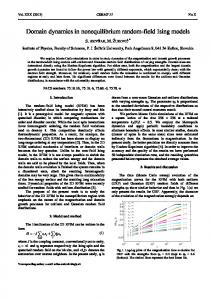
FIG. 1. (Color online) Time evolution of domains for a 128 × 128 system at T = 0.50. The strength of disorder is η0 = 1.0. The yellow (grey) regions indicate domains of up spins.
3 this spin contains a factor exp(−2β|ηi |), which is a very small number if |ηi | is large. It is said that the domain wall is pinned by the local field, i.e., it is prevented from moving by an energy barrier produced by the large random field. If the domains eventually stop growing, the system will be in a disordered phase (although the domain size may be very large). This describes the d = 2 RFIM. All these features can be visualized from some snapshots presented in Fig. 1. In the early time regime, domains begin to form and grow in size (Fig. 1 (a) (d)). This is seen in pure system too. As time flows, the domains stop growing and the domain wall is pinned (Fig. 1 (e) - (h)) even at a low temperature. The introduction of a local static random field term changes the behaviour of the system completely in later time regime and renders the system in a disordered phase even at a very low temperature. These disordered spin systems have been an active area of research for quite some time now [10–16]. The purpose of the present work is to study the disorder induced changes in the properties of these systems, with emphasis on the dynamical evolution of the domain growth, the order parameter and the spin-spin correlation functions in the non equilibrium region. In most of the studies on RFIM, the domain size (or the cluster size) was determined in terms of the fluctuations of the magnetization [17–21]. The fluctuations in magnetization is only a measure of domain size, not the actual domain size. In this work, we have measured the actual domain size by Hoshen-Kopelman algorithm [22]. The method of determining cluster size by Hoshen-Kopelman algorithm allows us to make a more accurate study of its growth with time. Moreover, there are many ways in which the random fields could be chosen. In most of the studies, they were chosen to have a Gaussian distribution with some finite width σ, or to have values randomly ±h where h is a constant. Although, the interesting properties of RFIM are believed to be independent of the exact choice of the distribution which is a consequence of the phenomenon of universality [23]. In the present work, the random fields are chosen from a uniform distribution of varying strengths. The rest of the paper is arranged as follows. Section II discusses the computational details and gives the definition of the thermodynamic quantities of our interest. Section III presents the results in detail. Finally in Section IV, we summarize our results.
II.
THE MODEL AND ITS SIMULATION
The first term of the Hamiltonian (1) is the usual exchange interaction term while the second term represents the interaction of the random field with the spin. We call this term the pinning interaction term since this term is responsible for domain wall pinning. The simulations are performed on square lattice of sizes ranging from 32 × 32
to 512 × 512 and at a finite temperature T = 0.50 which is well below the critical temperature of 2d zero field Ising model. The temperature is taken sufficiently low to reduce the thermal fluctuations. Properties of RFIM depend on the competition between the random fields and the ferromagnetic couplings with the thermal fluctuations serving only to renormalize the strengths of these couplings [24]. We have chosen Metropolis algorithm [25] to simulate the system. Metropolis algorithm is suitable here because the dynamics is local. Being a single spin flip dynamics, the Metropolis algorithm is believed to represent the natural way of evolution of a system, since the acceptance ratio is given by the Boltzmann Probability. Periodic boundary conditions (PBC) are used in the simulations. The sizes of the domains (or clusters) are determined by Hoshen-Kopelman (HK) algorithm [22]. The general idea of the HK algorithm is that we scan through the lattice looking for up spins (or down spins). To each up spin (or down spin) we assign a label corresponding to the cluster to which the up spin (or the down spin) belongs. If the up spin (or the down spin) has zero neighbours of same sign, then we assign to it a cluster label we have not yet used (it’s a new cluster). If the up spin (or the down spin) has one neighbour of same sign, then we assign to the current spin the same label as the previous spin (they are part of the same cluster). If the up spin (or the down spin) has more than one neighbour of same sign, then we choose the lowest-numbered cluster label of the up spins (or the down spins) to use the label for the current spin. Furthermore, if these neighbouring spins have different labels, we must make a note that these different labels correspond to the same cluster. The HK algorithm is a very efficient cluster identification method for twodimensional systems. The domain size corresponds to the number of spins enclosed by the boundary of a domain. The time dependent ensemble average of magnetization, i.e., the order parameter has been defined as 1 X M (η0 , t) = h 2 | si |it (2) L i where L is the linear size of the system and si is the spin at the site i. The angular bracket h· · · it indicates the ensemble average at time t. The time dependent ensemble average of the spin-spin correlation function is defined as ψss (η0 , l, t) = hhsi si+l il it
(3)
where l is the distance of separation between the spins. The angular bracket h· · · il indicates the ensemble average over the distance of separation between the spins while h· · · it indicates the same over time t. The thermodynamic quantities of our interest are averaged over 50 independent simulations to improve the accuracy and the quality of the results. The simulations start with a random spin configurations, characteristic of a high temperature phase and then quenched to a low temperature.
4 III.
0.5
RESULTS AND DISCUSSIONS
0.45
The dynamic evolution of the order parameter defined in Eq. (2) for different disorder strengths is shown in FIG. 2. It is seen from FIG. 2 that for weak disorder
0.4
β(η0)
0.35
100 η = 0.2 0 η0 = 0.3 η0 = 0.4 η0 = 0.6 η0 = 1.0 η0 = 1.4 η0 = 1.8 η0 = 2.2 η0 = 2.6 η0 = 3.0
0.3 0.25 0.2 0.15 0.1 0.05
M(η0,t)
10-1
0
0.5
1
1.5 η0
2
2.5
3
FIG. 3. (Color online) Variation of the exponent β(η0 ) with η0 . The solid line indicates the best exponential fit to the data points. 10-2 100
101
102
t
103
exchange interaction defined as X si sj it χ(η0 , t) = h
104
FIG. 2. (Color online) Plot of the time evolution of order parameter for L = 256. The dashed lines represent the best linear fits according to the scaling law defined in Eq. (4)
(η0 ≤ 0.3) the system reaches in a steady state after a certain time (here steady state means the fluctuations in order parameter is very small with time). For weak disorder, the system behaves more or less like a pure system. For larger disorder, the system takes longer time to reach in a steady state, i.e., the system relaxes, if at all, very slowly. The nature of the evolution of the order parameter strongly depends on the strength of the disorder. The early time behaviour of the dynamic evolution of the order parameter can be characterized by the following power law behaviour M (η0 , t) ∼ tβ(η0 )
(5)
hiji
as well as the time evolution of the time-dependent ensemble average of the normalized pinning interaction defined as Ω(η0 , t) = h
1 hsi ηi iit η0
(6)
where the angular bracket h· · · it indicates the ensemble average at time t. FIG. 4 shows the dynamic evolution of the χ(η0 , t) and the Ω(η0 , t) respectively and it reveals χ(η0,t)
100 Ω(η0,t)
(4) 10-1
where β(η0 ) is a disorder-strength-dependent exponent corresponding to the growth of the order parameter. The dependence of the power law exponent β(η0 ) on the disorder strength η0 is shown in FIG. 3. The exponent β(η0 ) falls off exponentially with the strength of the disorder η0 as ∼ exp(−νη0 ) with ν = 1.35 ± 0.07. This is quite obvious. Two types of interactions, namely, the exchange interaction and the pining interaction are present in the system. For larger disorder, spin flips are not favoured due to the presence of the pinning interaction term and consequently the domain walls get pinned, leaving the system in a disordered phase. As a result, the exponent β(η0 ) falls off sharply with η0 . What happens is that there is always a competition between the exchange interaction and the pining interaction. Therefore it is interesting to observe the time evolution of the time-dependent ensemble average of the
η0 = 0.2 η = 0.6
10-2 η0 = 1.0 0 η0 = 1.4 η0 = 1.8 η0 = 3.0
100
101
102
t
103
104
105
FIG. 4. (Color online) The time evolution of the exchange interaction χ(η0 , t) and the pinning interaction Ω(η0 , t) as defined in Eq. (5) and Eq. (6) respectively for L = 256.
a striking feature. It is seen that the exchange interaction χ(η0 , t) remains almost same with time except at some initial time steps whereas the pinning interaction Ω(η0 , t) decays more rapidly except for very large disorder strength. The system evolves with time in such
5 0.1
0.4 0.35
0.08 0.3 0.25
αχ(η0)
αΩ(η0)
0.06
0.04
0.2 0.15 0.1
0.02 0.05 0
0
0.5
1
1.5 η0
2
2.5
3
0
0
0.5
1
1.5 η0
2
2.5
3
FIG. 5. (Color online) Variation of αχ (η0 ) and αΩ (η0 ) with η0 .
a way that the pining interaction gets minimized. We would like to point out that this behaviour is characteristic to the RFIM and was not observed earlier to the best of our knowledge. For weak disorder, the system achieves the steady state with the flow of time resulting in the saturation of the pining interaction and the exchange interaction as well. For disorder strengths lying in the intermediate range, the decay of pining interaction strongly depends on the strength of the disorder. Now a natural question that arises is that how rapidly does the pining interaction Ω(η0 , t) decay or how slowly does the exchange interaction χ(η0 , t) increase with the strength of the random field η0 . According to the nature of the dynamic behaviour seen in FIG. 4, the power law dependence of the χ(η0 , t) and the Ω(η0 , t) with time has been proposed as χ(η0 , t) ∼ tαχ (η0 ) Ω(η0 , t) ∼ t
(7)
−αΩ (η0 )
where αχ (η0 ) and αΩ (η0 ) are two characteristic exponents which determine the nature of growth of the exchange interaction and the pining interaction. The variation of these exponents with η0 is shown in FIG. 5. The values of the exponent αχ (η0 ) are very small and its variation with the strength of the disorder η0 is negligible which indicate that αχ (η0 ) is almost independent of η0 . On the other hand, the variation of the exponent αΩ (η0 ) with η0 is noticeable and αΩ (η0 ) decreases rapidly with η0 and tends to saturate for very large values of η0 . These results confirm our earlier observation on the time evolution of the exchange interaction and the pinning interaction. Next we focus our attention on the study of spin-spin correlation functions defined by Eq. (3). The spin-spin correlation functions ψss (η0 , l) for different strengths of disorder at different times t are shown in FIG. 6. For weak disorder, when the system is quenched from a high temperature phase to a low temperature one, long range
order is seen to develop at later time regime. With decreasing strength of the random fields, the ferromagnetic couplings start to dominate over the random fields, the domains of parallel spins become larger and the system is in a ferromagnetic regime. This observation is in agreement with [26, 27] which shows that there is a critical field strength at which the correlation length becomes divergent. This observation also supports the earlier findings [7] of a phase transition in the 2d RFIM at T = 0. Here the thermal fluctuations due to finite temperature serves only to renormalize the strengths of the random fields and the ferromagnetic couplings. For weak disorder, the pinning interaction decays faster with time and then saturates (see FIG. 4), which also implies presence of long range order at later time regime. This is why, we obtained a large value of the exponents β(η0 ) and αΩ (η0 ) for weak disorder strengths. We would also like to point out here that with the increase in system size, it takes longer time in order for long range order to be established. To check that the presence of long range order for weak disorder is not a result of finite size effect, we have plotted the order parameter against time (the number of Monte Carlo steps) for various system sizes, which is shown in FIG. 7. It is evident from FIG. 7 that the number of Monte Carlo steps (tx ) required to achieve the long range order for weak disorder increases with the increase in system size. The inset of FIG. 7 shows the plot of ln(tx ) against ln(L). It may also be noted that for weak disorder, the nature of spin-spin correlation functions changes from exponential decay to power law decay at late time stage, which suggests the possibility of existence of long range order. This observation is in agreement with the recent observation of Aizenman [8]. For strengths of disorder lying in the intermediate range, no long range order is seen to develop and short range order is being developed with time in the system. Except for weak random fields, Exchange interaction never wins over pinning interaction to establish long range order in the
6 1
1
t = 10 t = 100 t = 1000 t = 10000 t = 100000
0.8
0.8
0.6
0.6 ψss(l)
ψss(l)
η0 = 0.2 0.4
0.2
0
0
0
50
100
150 l
200
250
1
300
-0.2
50
100
150 l
200
250
300
t = 10 t = 100 t = 1000 t = 10000 t = 100000
0.8
0.6
0.6 ψss(l)
η0 = 1.0 0.4
η0 = 2.6 0.4
0.2
0.2
0
0
-0.2
0
1
t = 10 t = 100 t = 1000 t = 10000 t = 100000
0.8
ψss(l)
η0 = 0.6 0.4
0.2
-0.2
t = 10 t = 100 t = 1000 t = 10000 t = 100000
0
50
100
150 l
200
250
300
-0.2
0
50
100
150 l
200
250
300
FIG. 6. (Color online) Plot of ψss (η0 , l) against l for different disorder strengths at different times for L = 512.
10
η0 = 0.20
10
12 10
-2
L=32 L=64 L=128 L=192 L=256 L=512
-3
10
0
10
1
ln(tx)
10
ever, the presence of random fields prevents the system from growing into a single domain even at a low temperature. For very large disorder (≥ 2.6), neither short range order nor long range order prevails in the system and the system remains in a complete disordered phase. There is always a competition between the ferromagnetic nearest neighbour interaction J (which favours ordering) and the random field strength η0 (which favours disordering). In the limit of strong random fields, the direction of spins follows the direction of random fields.
-1
M(η0,t)
10
0
8 6 4
10
2
10
3
3
4
5 ln(L)
10
6
4
7
10
5
t
FIG. 7. (Color online) Plot of the order parameter against time for various system sizes at η0 = 0.20.
system. Due to this short-range order, there forms small domains in the system initially and as time elapses, these small domains “evaporate” to form a large domain. How-
Now we present the results of the domain growth with time. Domain growth in quenched non equilibrium systems is a widely studied topic [28]. Monte Carlo simulations have been carried out [29–32] to obtain numerically the time evolution of these domains, and to compare the results with theory [33–36]. We concentrate on the growth of the largest domain and it is plotted in FIG. 8. The growth of the largest domain can be characterized by the following power law behaviour :
7 the values of the exponents are different and the fall of µ(η0 ) is faster than that of β(η0 ).
0.9
η0 = 0.2 η0 = 0.3 0.8 η0 = 0.4 η0 = 0.6 η0 = 1.0 0.7 η0 = 1.4 η0 = 1.8 η0 = 2.6
IV.
SUMMARY AND CONCLUSION
Λ(η0,t)
0.6
0.5
0.4 101
102
t
103
104
105
FIG. 8. (Color online) Plot of the growth of the largest domain of the system with time for L = 256. The dotted lines represent the best linear fit to the data points.
For η0 ≤ 0.3 Λ(η0 , t) = tµ(η0 )
t ≪ t×1
ν(η0 )
t× 1 ≪ t ≪ t× 2 t ≫ t× 2
Λ(η0 , t) = t Λ(η0 , t) = η0σ
(8)
For η0 > 0.3 Λ(η0 , t) = tµ(η0 )
(9)
where µ(η0 ) is a disorder-strength-dependent exponent corresponding to the growth of the largest domain at the early time regime. Recently, Corberi et. al. [37] also found that the domain growth shows a power law scaling with a disorder dependent exponent in preasymptotic regime. The variation of the exponent µ(η0 ) with η0 is shown in FIG. 9. The exponent µ(η0 ) falls off exponen0.08 0.07 0.06
µ(η0)
0.05 0.04 0.03 0.02 0.01 0
0
0.5
1
1.5 η0
2
2.5
We conclude the paper with a summary of our results. This paper has attempted to consider some aspects of the non equilibrium behaviour of the 2d random-field Ising model numerically at a low temperature. As seen in the preceding Sections, the RFIM exhibits a variety of behaviours depending on the strength of the random fields. The system relaxes with time in presence of two opposite kind of interactions, namely the exchange interaction and the pinning interaction and we have studied the dynamical evolution of these two interactions separately. It is seen that the fall of pinning interaction depends on the strength of the random fields with a power law decay and it decays faster for weak random fields. Therefore the dynamical evolution of the order parameter should also depend on the strength of the random fields with a power law growth, as has been observed. To get an insight of what is happening inside the system, we have calculated the dynamical spin-spin correlation functions. For weak disorder, the pinning interaction decays faster and consequently the disordering effect reduces. As a result, the system is being correlated with time for weak disorder. Our numerical study suggests the possibility of presence of long range order in the 2d RFIM for weak disorder strengths. We are inclined to comment that the 2d RFIM exhibits a phase transition in disorder parameter even at a temperature T > 0. The transition is manifested by a change of nature of spin-spin correlation functions from an exponential decay at high disorder strengths to a power law decay at weak disorder strengths. The thermal fluctuations due to non zero T plays the role only to renormalize the strengths of both the interactions, although it ceases to be of relevance at higher temperatures. Except for weak disorder, the exchange interaction never wins over the pinning interaction to establish long range order in the system. The study of spin-spin correlation functions reveals that the 2d RFIM shows long-range order, short-range order and no order at all, each of which occurs in a restricted range of random field strength. We have also measured the largest cluster size by using the Hoshen-Kopelman algorithm. The behaviours of the dynamical evolution of the largest cluster are consistent with our previous conclusions.
3
FIG. 9. (Color online) Plot of the exponents µ(η0 ) with disorder strength η0 .
tially with the strength of disorder η0 as ∼ exp(−γη0 ) with γ = 1.92 ± 0.14. It is to be noted that although the order parameter exponent and the domain growth exponent fall off exponentially with the strength of disorder,
V.
ACKNOWLEDGEMENTS
One of the authors (SS) acknowledges support from the UGC Dr. D. S. Kothari Post Doctoral Fellowship under grant No. F.4-2/2006(BSR)/13-416/2011(BSR). SS also thanks Heiko Reiger for many useful discussions. The authors acknowledge S. M. Bhattacharjee for a careful
8 reading of the manuscript and a number of comments.
The authors thank the anonymous referee for a number of suggestions in improving the manuscript.
[1] Y. Imry and S. K. Ma, Phys. Rev. Lett 35, 1399 (1975). [2] D. P. Belanger, A. R. King and V. Jaccarino, Phys. Rev. B 31, 4538 (1985); Phys. Rev. Lett. 54, 577 (1985). [3] G. Grinstein and D. Mukamel, Phys. Rev. B 27, 4503 (1983). [4] G. Parisi and N. Sourlas, Phys. Rev. Lett 43, 744 (1979); A. P. Young, J. Phys. C 10, L257 (1977). [5] J. Bricmont and A. Kupiainen, Phys. Rev. Lett 59, 1829 (1987). [6] M. Aizenman and J. Wehr, Phys. Rev. Lett 62, 2503 (1989); 64, 1311 (1990). [7] C. Frontera and E. Vives, Phys. Rev. E 59, 1295(R) (1999). [8] See the talk at http://ricerca.mat.uniroma3.it/ipparco/ convegno70/seminars.html [9] D. Spasojevic, S. Janicevic and M. Knezevic, Phys. Rev. Lett 106, 175701 (2011). [10] D. Spasojevic, S. Janicevic and M. Knezevic, Phys. Rev. E 84, 051119 (2011). [11] M. Tissier and G. Tarjus, Phys. Rev. Lett 107, 041601 (2011). [12] R. L. C. Vink, T. Fischer and K. Binder, Phys. Rev. E 82, 051134 (2010). [13] B. Cerruti and E. Vives, Phys. Rev. E 80, 011105 (2009). [14] N. J. Zhou, B. Zheng, and Y. Y. He, Phys. Rev. B 80, 134425 (2009). [15] F. Colaiori et. al., Phys. Rev. Lett. 92, 257203 (2004). [16] R. Paul, G. Schehr, and H. Rieger, Phys. Rev. E 75, 030104(R) (2007). [17] S. R. Anderson, Phys. Rev. B 36, 8435 (1987). [18] E. T. Gawlinski, K. Kaski, M. Grant, and J. D. Gunton, Phys. Rev. Lett. 53, 2266 (1984).
[19] E. T. Gawlinski, S. Kumar, M. Grant, and J. D. Gunton, and K. Kaski, Phys. Rev. B 32, 1575 (1985). [20] D. Chowdhury and D. Stauffer, Z. Phys. B 60, 249 (1985). [21] A. Sadiq and K. Binder, J. Stat Phys. 35, 517 (1984). [22] H. Hoshen and R. Kopelman, Phys. Rev. B 14, 3438 (1976). [23] Monte Carlo methods in Statistical Physics, edited by M. E. J. Newman and G. T. Barkema, (Clarendon, Oxford, 1999). [24] Y. Wu and J. Machta, Phys. Rev. Lett 95, 137208 (2005). [25] N. Metropolis et. al., J. Chem. Phys. 21, 1087 (1953) [26] E. T. Seppala and M. J. Alava, Phys. Rev. E 63, 066109 (2001). [27] L. Kornyei and F. Igloi, Phys. Rev. E 75, 011131 (2007). [28] A. J. Bray, Adv. Phys. 43, 357 (1994). [29] D. Stauffer, C. Hartztein, K. Binder and A. Aharony, Phys. Condens. Matter 55, 325 (1984). [30] M. Grant and J. D. Gunton, Phys. Rev. B 29, 1521 (1984). [31] E. Pytte and J. F. Fernandez, Phys. Rev. B 31, 616 (1985). [32] J. L. Cambier and M. Nauenberg, Phys. Rev. B 34, 7998 (1986). [33] J. Villain, Phys. Rev. Lett 52, 1543 (1984). [34] G. Grinstein and J. R. Fernandez, Phys. Rev. B 29, 6389 (1984). [35] H. Yoshisawa and D. P. Belanger, Phys. Rev. B 30, 5220 (1984). [36] R. Bruinsma and G. Aeppli, Phys. Rev. Lett 52, 1547 (1984). [37] F. Corberi et. al., Phys. Rev. E 85, 021141 (2012).