Three-dimensional direct numerical simulations of the full compressible Navierâ ... to reasonable agreement between experiments and numerical simulations.
AIAA 2007-3405
13th AIAA/CEAS Aeroacoustics Conference (28th AIAA Aeroacoustics Conference)
Direct Numerical Simulations of Three-Dimensional Cavity Flows Guillaume A. Br`es∗ and Tim Colonius† California Institute of Technology, Pasadena, CA 91125, U.S.A. Three-dimensional direct numerical simulations of the full compressible Navier–Stokes equations are performed for cavities that are homogeneous in the spanwise direction. The formation of oscillating spanwise structures is observed inside the cavity. We show that this 3D instability arises from a generic centrifugal instability mechanism associated with the mean recirculating vortical flow in the downstream part of the cavity. In general, the threedimensional mode has a spanwise wavelength of approximately 1 cavity depth and oscillates with a frequency about an order-of-magnitude lower than 2D Rossiter (flow/acoustics) instabilities. The 3D mode properties are in excellent agreement with predictions from our previous linear stability analysis. When present, the shear-layer (Rossiter) oscillations experience a low-frequency modulation that arises from nonlinear interactions with the three-dimensional mode. We connect these results with the observation of low-frequency modulations and spanwise structures in previous experimental and numerical studies on open cavity flows. Preliminary results on the connections between the 3D centrifugal instabilities and the presence/suppression of the wake mode are also presented.
I. A.
Introduction and previous work
Motivations
The flow over a cavity gives rise to a wide range of flow phenomena and remains a challenging problem for control. In compressible flow, cavity oscillations arise from a flow-acoustic resonance mechanism involving (i) shear layer amplification of disturbances, (ii) generation of acoustic waves upon impingement of vortical disturbances on the downstream edge of the cavity, and (iii)upstream propagation and conversion of pressure waves into vortical waves near the upstream corner, providing further instabilities in the shear layer. This feedback process can lead to resonance and self-sustained oscillations. This type of flow is referred to as shear-layer (Rossiter1 ) mode, from the early work of Rossiter who developed the now classic semi-empirical formula to predict the resonant frequencies: Stn =
n−α fn L = U M + κ1
n = 1, 2, 3...
(1)
where Stn is the Strouhal number corresponding to the n-th mode frequency, fn , κ and α are empirical constant corresponding to the average convection speed of the vortical disturbances in the shear layer, and a phase delay. Apart from the instability mechanism proposed by Rossiter, another mode of oscillation have been observed in a few cavity flow experiments.2 In this mode, the flow is characterized by a large-scale vortex shedding from the cavity leading edge, similar to that observed behind bluff bodies, hence the term “wake mode” used to describe the resulting flow regime. As the large vortex (dimension of the cavity depth) forms near the leading edge, free stream fluid enters the cavity and impinges on the cavity bottom. The vortex is then shed from the leading edge and is violently ejected from the cavity, the all process resulting in a drastic increase in drag. ∗ Ph.D.,
Mechanical Engineering, California Institute of Technology, Pasadena, CA, Student Member AIAA Mechanical Engineering, California Institute of Technology, Pasadena, CA, Member AIAA
† Professor,
1 of 16 American Institute of Aeronautics and Astronautics Copyright © 2007 by G.A. Brès & T. Colonius. Published by the American Institute of Aeronautics and Astronautics, Inc., with permission.
The wake mode transition has been observed in several two-dimensional numerical simulations,3–6 but experimental evidence of this mode is limited. Three-dimensionality has been shown to play a role in suppressing the wake mode. For instance, two-dimensional cavities oscillating in wake mode return to shear-layer mode when random three-dimensional inflow disturbances are introduced.7, 8 These studies show again how a better understanding of the fundamental three-dimensional features of cavity flows is crucial to accurately connect numerical results, experiments and practical applications. Since the earlier work of Rossiter, two-dimensional cavity flows have received significant attention, leading to reasonable agreement between experiments and numerical simulations. In comparison, three-dimensional cavity flow remains a challenging subject, still highly relevant for practical applications. While observations of three-dimensionality have been reported in cavity flow experiments,9–11 the physics of these features has yet to be fully understood. As a result, past efforts on cavity flow control have typically ignored non-parallel and three-dimensional effects. These approaches may, on one hand, reduce the effectiveness of model-based control, or on the other hand disregard important three-dimensional mechanisms that could be exploited in passive ways to reduce broadband noise. To investigate these issues, we perform Direct Numerical Simulations (DNS) of the nonlinear compressible Navier–Stokes equations for selected 3D cavity configurations, based on the results of our previous three-dimensional linear stability analysis.12, 13
B.
Numerical methods
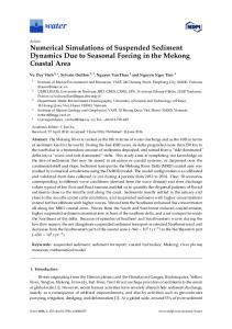
Following previous work on cavity flows,5 we developed a DNS code12, 13 to solve the full compressible Navier–Stokes (NS) equations and study the flow over three-dimensional open cavities. A linearized version of the equations was also implemented, and the existing DNS code can solve linear or nonlinear NS equations for both 2D or 3D flows. The cavity is supposed homogeneous (periodic) in the spanwise direction (z-direction). The code can handle any type of block geometry (including the rectangular cavity shown in figure 1) and is fully parallelized using Message-Passing Interface (MPI). The cavity configuration and flow conditions are controlled by the following parameters: the cavity aspect ratio L/D and spanwise wavelength Λ/D, the ratio of the cavity length to the initial boundary layer momentum thickness at the leading edge of the cavity L/θ0 , the Reynolds number Reθ = U θ0 /μ and the freestream Mach number M = U/a∞ .
Buffer zone Outflow
Inflow
Outflow
U
ș
Λ
D
y z
x
L
Figure 1. Schematic diagram of the computational domain
2 of 16 American Institute of Aeronautics and Astronautics
C.
Linear stability results
The linear stability analysis is presented in details in our previous papers12, 13 and is conducted as follow: given a cavity configuration and flow conditions, a two-dimensional simulation is performed. For subcritical condition (i.e., the self-sustained oscillations are damped), the 2D steady flow is extracted from the DNS and used as base flow for the linear 3D simulations. A perturbation of given spanwise wavelength λ is added to the 2D steady base flow as initial condition, and the 3D linear Navier–Stokes equations are solved to investigate the cavity response. Under most conditions, there is a single dominant mode in the long-time behavior of the cavity flow for a given spanwise wavelength. The growth rate and frequency of the resulting mode can then be determined. The results of the linear stability analysis are summarized here, as they are the starting point of the present work: 1. For several different cavity configurations and flow conditions, the least damped 3D mode is unstable and exhibits similar features in terms of wavelength and flow structure in all cases. For a band of spanwise wavelength around the size of the cavity depth (λ/D ≈ 1), an instability would develop in the cavity, which is characterized by a growing disturbance oscillating in the recirculating vortical flow (also referred to as primary vortex) in the downstream half of the cavity. This mode is referred to as mode ii. 2. Typically, the unsteady three-dimensional instabilities have a frequency about an order of magnitude lower than the two-dimensional shear-layer (Rossiter) oscillation frequency. We show that the 3D mode frequency is related to the time for disturbances to advect around the recirculating region. 3. The Mach number appears to have little influence on the growth rate and frequency of the dominant mode. This observation indicates that the instability is not acoustic but hydrodynamic in nature. 4. On the other hand, the influence of the Reynolds number is significant, that is, the linear growth rate of the 3D instability increases with Reynolds number. This results indicates that there is a critical Reynolds number, above which the flow becomes 3D unstable. 5. Ultimately, we show that the instability mechanism is the generic centrifugal instability associated with the closed streamlines in the recirculating vortical flow near the downstream cavity wall. This centrifugal instability is similar to the one previously identified in flows over a backward-facing step, lid-driven cavity, and Couette flows. A steady mode of smaller spanwise wavelength 0.4D was also identified for a shorter cavity with L/D = 1. We argue that the specific properties of the three-dimensional mode for the square cavity are related to the primary vortex that occupies the whole cavity in that particular configuration. This mode, referred to as mode i, is not the focus of the present work.
II.
Nonlinear Three-Dimensional Simulations
To investigate the effect of these instabilities on real flows, full three-dimensional nonlinear simulations are performed. Both subcritical (run 2M0325-3D) and supercritical conditions (runs 2M06-3D) are considered. For the 3D simulations, the steady (or time-averaged) basic state extracted from the two-dimensional DNS data is perturbed by small disturbances of spanwise wavelength λ/D = 2 and λ/D = 1, corresponding to the first two spanwise wavenumbers in the 3D simulation. The full NS equations are then numerically solved on a homogeneous three-dimensional cavity of spanwise extent Λ/D = 2. As the linear stability results suggest that the spanwise wavelength of the dominant 3D mode is in the range 0.4 ≤ λ/D ≤ 1.25, such cavity aspect ratio is expected to be sufficient to capture all the flow physics. For the cavity of aspect ratio L/D = 2, the grid contains about seven and a half million grid points, with (N x = 120, N y = 60, N z = 128) points across the cavity in the streamwise, depth and spanwise directions, respectively. In each case, the computational domain extends several cavity depths upstream, downstream, and above the cavity.
3 of 16 American Institute of Aeronautics and Astronautics
A.
Subcritical conditions
The first configuration considered is the subcritical run 2M0325, for a cavity of aspect ratio L/D = 2 at low Mach and Reynolds number (M = 0.325, ReD = 1500, L/θ0 = 53). The two-dimensional simulation shows that the flow is initially oscillating at a frequency StD = f D/U = 0.241 close to Rossiter first mode, with exponentially decaying amplitude, and ultimately converges to a steady state. Run L/D ReD L/θ0 M Rossiter prediction
2M0325 2D subcritical 2 1500 52.3 0.325 StD Mode λ/D 0.181 I ∞ 0.422 II ∞
2D DNS
0.241†
I
∞
3D Linear Stability
0.025 0.240†
ii I
1 ∞
3D DNS
0.025 0.240†
ii I
1 ∞
2M06 2D supercritical 2 1500 52.3 0.6 StD Mode λ/D 0.160 I ∞ 0.372 II ∞ 0.204
I
∞
n.a. n.a. 0.026 0.352
ii II
1 ∞
Table 1. Comparison of the dominant mode prediction for 2D and 3D runs with L/D = 2. Only the most energetic frequencies StD = f D/U for the cavity flows are presented, along with the spanwise wavelength λ/D of the instability. The original values from Rossiter (1/κ = 1.75, α = 0.25) were used in the semi-empirical formula in equation 1. † For subcritical conditions, the Rossiter modes are damped but the oscillation frequency can still be measured from the early times. The linear stability results are not available (n.a.) for supercritical conditions.
Figure 2(a) shows a portion of the time-history of the velocity v/U for both 2D and 3D simulations at approximately the same location in the middle of the cavity. Initially, the three-dimensional flow oscillates at a frequency corresponding to the 2D Rossiter mode. This frequency and its first harmonic are evident in the spectrum in figure 2(b). After a transition period, the 2D modes decay while the 3D mode grows and saturates. The final frequency of oscillation is StD = 0.025 corresponding to the frequency of the most unstable three-dimensional mode from the linear stability analysis (see table 1). As the shear-layer oscillations are damped and eventually die out, the three-dimensional instability associated to the centrifugal mechanism is the only unsteady feature remaining in the flow: the growth and decay of disturbances rotating around the primary vortex can be observed in the cavity, as can the formation of a cellular pattern (see figure 3) similar to the linear stability results. As predicted, the spanwise wavelength of the 3D mode is equal to one cavity depth. Here, we conclude that the mode ii predicted by the linear stability analysis13 is observed in the 3D nonlinear simulation. Under the present conditions, the three-dimensional instability remains weak and is mainly active in the recirculating region within the cavity. The interaction with the shear layer is also weak and mostly limited to a low-frequency, small-amplitude oscillation.
4 of 16 American Institute of Aeronautics and Astronautics
v/U
0.02
0.01
v/U (Power spectrum magnitude)
200 0.02
0
Mode ii
10−2
Mode I
10−4
0.01 0
0
10−6
0
200
400
tD/U (a)
600
800
1000
0
0.2 0.4 0.6 0.8 StD (b)
1
Figure 2. (a) Time trace of normal velocity at (x, y) = (0.5L, 0) for 2D run 2M0325 ( ) and 3D run 2M0325-3D ( ) at z = 0. The other flow variables exhibit the same characteristics. To show all the data clearly, the bottom and left axes correspond to the 3D simulation, and the top and right axes to the 2D run. (b) Spectrum of the normal velocity presented in (a). The different modes are identified and their harmonics can also be observed
B.
Supercritical conditions
Supercritical conditions are obtained from the previous simulations by simply increasing the Mach number from M = 0.325 to M = 0.6 while keeping the other parameters constant. In run 2M06, the two-dimensional flow exhibits disturbances of growing amplitude and eventually saturates into a periodic oscillating flow of frequency corresponding to the Rossiter mode I. In this case, a time-averaged steady state is extracted by averaging the periodic data and the 3D nonlinear simulation is performed following the same procedure as the subcritical case. 1.
Unsteady flow structure
The flow structure is shown in figure 3 for comparison with the subcritical case 2M0325-3D. Both flows exhibit identical three-dimensional features in terms of cellular pattern inside the cavity and oscillation frequency. The velocity field in the cavity is stronger in this case and this increase leads to larger iso-surfaces in figure 3. The dominant spanwise wavelength is still λ/D = 1. Here, the 3D instability can again be identified with mode ii.
(a)
(b)
Figure 3. Visualisation of the instantaneous spanwise structures: (a) 3D run 2M0325-3D; (b) 3D run 2M06-3D. The iso-surfaces represent the spanwise velocity levels w/U = −0.01 and w/U = 0.01. The whole spanwise extent of the cavity is shown and the wavelength λ/D = 1 of the instability can clearly be observed. The velocity vectors in the streamwise cross-section at z = 0 are shown inside the cavity and once in the freestream for comparison.
5 of 16 American Institute of Aeronautics and Astronautics
For these supercritical conditions, shear-layer oscillations are also present in the 3D simulations and the interaction between the three-dimensional instabilities and the shear layer is significant. In the downstream half of the cavity, the spanwise structures enter the shear layer and impinge on the downstream edge. Part of the disturbances is swept downstream while the other part goes back into the recirculating flow inside the cavity. In general, the spanwise wavelength λ/D = 1 of these structures can still be observed as they are convected downstream of the cavity. Experimental evidence of the spanwise structures we observed in our simulations can be found in the recently published work by Faure et al..11 They performed low speed experiments for open cavities of aspect ratio L/D = 0.5 to 2 at medium range Reynolds numbers, with laminar incoming boundary layers. Smoke is used for flow visualisations. Under certain conditions, they observe the formation of “mushroom-like counterrotating cells” near the upstream wall and symmetrically at the downstream wall. Their measurements are in good agreement with our results, bot in terms of spanwise wavelength and critical Reynolds number of the 3D instability. 2.
Oscillation frequencies
The time-history of the streamwise velocity u/U for runs 2M06 and 2M06-3D are compared in figure 4. It is interesting to note that both Rossiter modes I and II are initially unstable in the two-dimensional simulation, but through a process of nonlinear amplification and saturation, mode I is selected, while mode II is damped and vanishes. In the three-dimensional simulation, after some transient exhibiting both Rossiter modes I and II, the self-sustained oscillations in the flow saturate into a periodic regime where the Rossiter mode II and the three-dimensional instability can be observed simultaneously. The different mode frequencies are reported in table 1. Since the 2D flow is supercritical, linear results for run 2M06 are not available for direct comparison with the three-dimensional mode frequency observed here. However, the low frequency measured here matches the predicted result from the linear stability analysis of run 2M0325 and the 3D mode frequency from run 2M0325-3D. There is no contradiction here, since we showed that the Mach number has little influence on the characteristics of the three-dimensional mode. This result is encouraging, as it tends to indicate that linear results from subcritical cases (if such stable conditions exist) could deliver useful insight on the 3D stability at higher Mach number for corresponding supercritical conditions. 0
400
350
400
u/U
0.2 0.1 0.2 0.1 0
tD/U (a)
700
650
tD/U (b)
700
Figure 4. (a) Time trace of streamwise velocity at (x, y) = (0.5L, 0) for 2D run 2M06 ( ) and 3D run 2M06-3D ( ) at z = 0.25D; (b) Details of the signal in the boxes in (a). To show all the data clearly, the bottom and left axes correspond to the 3D simulation, and the top and right axes to the 2D run.
In figure 4, it is clear that, in the three-dimensional simulation, the shear-layer oscillations exhibit a low-frequency modulations related to the 3D mode. The low-frequency peaks are observed in the power spectrum in figure 5. Similar results are obtained for the normal and spanwise velocities. For the present conditions, the peak associated with the 3D mode is in general about the same energy level or higher than the one for the Rossiter mode in the power spectra of the velocity field components. The low-frequency modulation is less evident in the time trace of the pressure. Here, we argue that the interaction between the 6 of 16 American Institute of Aeronautics and Astronautics
u/U (Power spectrum magnitude)
10
0
Mode ii
Mode II
10−2
10−4
0 Figure 5. 2M06 ( observed.
Mode I
0.2
0.4 0.6 StD
0.8
1
Power Spectrum of the periodic data of the streamwise velocity presented in figure 4: 2D run ); 3D run 2M06-3D ( ). The different modes are identified and their harmonics can also be
Rossiter mode and the three-dimensional instability is stronger for the velocity field than for the acoustic field because of the hydrodynamic nature of the 3D mode. Overall, these results are consistent with the present hypothesis that the 3D modes are related to the centrifugal instability mechanism. The low-frequency modulations is one characteristic feature of the unsteady three-dimensional mode that has been observed in experiments.14–16 Because this frequency is about an order of magnitude lower than the typical Rossiter mode frequencies, it is often not measured because of lack of resolution, and when it is, we believe the measurements tend to be overlooked or misinterpreted as caused by the experimental setup (such as fan noise, etc.). Based on our results, we propose here a different interpretation of the low-frequency modulation observed in experiments: namely, that it is caused by the centrifugal instability. Evidence of low-frequency peaks related to the three-dimensional centrifugal instability is also found in recent numerical work17, 18 for incompressible flows over open cavities. 3.
Time-averaged flow properties
Another key feature is that the shear-layer oscillation frequency now corresponds to the Rossiter mode II, rather than mode I as is selected in strictly two-dimensional simulations. To better assess the instability u(x, y)/dy)max is computed, where u ¯(x, y) properties of the shear layer, the vorticity thickness δω (x) = U/(d¯ is the time (and spanwise) average of the streamwise velocity. The vorticity thickness and its slope dδω /dx are typically used to measure the shear-layer spreading rate. Most researchers report that shear layer over open cavities exhibits approximately linear growth, much like free shear layers. However, the basic physics of these flows differs in two main aspects: that is, the shear layer is subject to a strong acoustic feedback, and the presence of the recirculating vortical flow in the downstream part of the cavity affects the entrainment and alters the shear-layer thickness. In both runs 2M06 and 2M06-3D, the shear layer initially exhibits linear growth, but there is a 15% decrease in the spreading rate between the 2D (dδω /dx ≈ 0.08) and 3D (dδω /dx ≈ 0.07) simulations. These results are of the same order as the spreading rates measured in experiments19 and numerical simulations.5 Typically, larger shear-layer spreading rates are obtained as L/θ0 is increased, and ultimately lead to higher dominant mode. In the present case, an increase in shear-layer spreading rate does not seem to be the cause of the higher mode observed in the three-dimensional simulation, as the opposite trend is be observed. The shear-layer measurements are consistent with other observations in the flow field. Here, we argue that the decrease in shear-layer spreading rate is related to the smaller oscillation amplitude and weaker recirculating region in the three-dimensional simulations. As shown in figure 4, the oscillation amplitude of the limit cycle slightly decreases between the 2D and 3D simulations. The mean velocity field inside the cavity 7 of 16 American Institute of Aeronautics and Astronautics
is also overestimated: for the three-dimensional computation, the spanwise-averaged velocity magnitude of the primary vortex is less than half of the two-dimensional prediction. Overall, the flow variables in the cavity are overestimated by about 5 to 10% of the freestream quantities. Likewise, observed, especially in the shear layer. Figure 6 shows √ a decrease in all√the Reynolds stresses is √ � � � � urms = u u /U , vr ms = v v /U , and wr ms = w� w� /U for the runs 2M06 and 2M06-3D. Here, the superscripts “ ¯ ” and “ � ” denote the time averaging and the fluctuating component of the flow variable with respect to the corresponding time-averaged quantity. The highest levels of urms are found in the shear layer in the downstream half of the cavity where the amplitude of oscillation is larger. For vrms , the highest levels are located near the downstream edge of the cavity because of the impingement process. The maximum amplitude of the rms velocity components are respectively 0.13 and 0.17 in the streamwise and normal direction for the 2D simulation. These maxima decrease to 0.1 and 0.12 in the 3D simulation. The quantity wrms has smaller values than the other rms velocities. The maximum amplitude is approximately 0.04 near the downstream wall because of the centrifugal instability mechanism.
√ u� u� /U
y
1
1
0
0
-1 √ v � v � /U
y
0
-1
4
2
1
1
0
0
-1
0
x
2
-1
4
0
2
4
0
2
4
2
4
1
√ w� w� /U
y
0 -1
(a)
0
x (b)
� � � Figure 6. Reynolds stresses u� u� /U , v� v� /U and w � w � /U (from top to bottom): (a) 2D run 2M06; (b) 3D run 2M06-3D. Five equi-spaced contours between 0.02 and 0.1 are represented. The spanwise average is shown for the 3D case.
The sound pressure levels (SPL) for the acoustic field above and inside the cavity in runs 2M06 and 2M06-3D are shown in figure 7. While the sound directivity is similar in both cases, with a peak radiation in the far field at about 135◦ from the downstream direction, the levels are in general lower for the 3D simulation. A noise reduction of about 5 dB can be observed in the far field, and up to 12 dB inside the cavity. This result is related to the decrease in oscillation amplitude previously mentioned. It is also in agreement with the general experimental observation that two-dimensional cavities are slightly louder than their three-dimensional counterparts. The weakened shear-layer coherence caused by turbulence is typically viewed as the key point to explain this experimental trend. A similar argument can be made here, even at lower Reynolds number. As the three-dimensional centrifugal instability establishes itself inside the cavity, the shear layer above develops the same spanwise fluctuations. This result can be seen in the contours of the vorticity magnitude presented in figure 8. Spanwise modulations are present in the shear-layer, starting around x = D. The resulting reduced spanwise coherence of the vortical structures traveling downstream in the shear layer affects the receptivity of the cavity trailing edge, which, in turn, reduces the acoustic scattering, the leading edge reinforcement of disturbances, and the overall effectiveness of the feedback process.
8 of 16 American Institute of Aeronautics and Astronautics
148
4
(a)
y
2
150
15
2 15
4
146
150 2 16
148
150
148
8 160
15
156
152
6
0
154 160 158
15
158
-2
0
6
146
148
y
4
146
4
(b)
2 x
2 148
14
150
8
15 146
1
-2
160 158
58
156 154
150
152
148
146
148
152
0
146
0
0
2 x
4
6
Figure 7. Sound pressure levels (SPL): (a) 2D run 2M06; (b) 3D run 2M06-3D. The spanwise average of the SPL is shown in this case.
9 of 16 American Institute of Aeronautics and Astronautics
4.
Discussion of the change in oscillation frequency
The change in mode frequency still needs to be addressed. A closer inspection at the spanwise vorticity for the 2D simulation 2M06 shows that only one vortex is present at a time in the shear layer across the cavity in agreement with the predicted Rossiter mode I. In contrast, two vortices can in general be observed simultaneously in the vorticity contours along the cavity, in any streamwise cross-section of the threedimensional simulation 2M06-3D. Looking at the evolution in time of the vorticity in both cases, it appears that the existence of the additional vortex, and therefore the shift in Rossiter mode, is caused by the presence of the three-dimensional instability. Disturbances rotating around the primary vortex in the downstream half of the cavity interact with the shear layer around x = 0.5L, likely leading to the change in the streamwise wavelength from λx /L = 1 to λx /L = 0.5.
(a)
(d)
(b)
(e)
(c)
(f)
Figure 8. Vorticity field for 3D run 2M06-3D. Six different times (a-f) are shown, corresponding to approximately one-sixth phase intervals of a half-period of the 3D instability. Five equi-spaced translucent iso-surfaces of the vorticity magnitude are represented for ||ω||D/U = 1 to 5.
In conclusion, both shear-layer oscillations and 3D mode are observed in the nonlinear simulation for the supercritical conditions of run 2M06-3D. Much like the previous case 2M0325-3D, spanwise structures of wavelength λ/D = 1 form inside the cavity and the three-dimensional mode corresponds to mode ii predicted by the linear stability analysis. Overall, the 2D simulation overestimates the amplitude of the shear-layer oscillations and of the flow field inside the cavity. Also, the shear-layer oscillations switch from Rossiter mode I (in the 2D simulations) to mode II, and experience a low-frequency modulation caused by the presence of the 3D mode. The results suggest that the interactions between the 2D and 3D modes seem to lead to the selection of that particular Rossiter frequency. Such observation could potentially be used to shed some light on the physics of mode selection in self-sustained oscillations. 10 of 16 American Institute of Aeronautics and Astronautics
III.
Wake mode
As mentioned in the introduction, another mode of cavity flow oscillation, commonly referred to as “wake mode,” has been observed in a few experiments2 and several two-dimensional numerical simulations.3–6 This mode is of interest here because three-dimensionality has been shown to play a role in its suppression.7, 8 We present here some preliminary results from ongoing work on the connections between the 3D centrifugal instabilities and the wake mode. A.
Two-dimensional simulation
The wake mode is characterized by the periodic shedding of a large vortex (about the size of the cavity) from the cavity leading edge, resulting in a significant increase in drag. Detailed description of the wake mode properties can be found in a recent article by Rowley et al..5 As Rowley et al.5 predicted the flow transition to wake mode for longer cavities and larger Mach and Reynolds number, we consider run 2M06 and increase the aspect ratio to L/D = 4 while keeping the other parameters constant. As expected, the resulting two-dimensional simulation 4M06wake (L/D = 4, M = 0.6, L/θ0 = 105.6, ReD = 1500) shows that the 2D flow oscillates in wake mode. The time-trace of the pressure, the streamwise and normal velocities are presented in figure 9(a), and are significantly different from the typical shear-layer mode results. The amplitude of oscillation is larger and the frequency is lower. The power spectrum in figure 9(b) shows that the oscillation frequency is StD = 0.063. This value is identical to those obtained by Rowley et al.5 for L/D = 4 cavities with Mach number within the range 0.4 < M < 0.8. In particular, StD = 0.064 for their run L4 with similar flow conditions. The power spectrum levels are about two orders of magnitude higher in this case, compare to the shear-layer mode. Overall, the large-scale shedding in the wake mode is a more violent event than the shear-layer oscillations.
0.5
0
-0.5 400
420
440
460
480
v/U (Power spectrum magnitude)
1 10
2
10
1
10
0
Wake mode
10−1
tU/D (a)
0
0.2
0.4 0.6 StD
0.8
1
(b)
Figure 9. (a) Time trace at (x, y) = (0.5L, 0) for 2D run 4M06wake: ( ) streamwise velocity u/U , ( ) normal velocity v/U , ( ) pressure P − P∞ ; (b) Spectrum of the normal velocity for 2D run 4M06wake. The wake mode frequency is identified and the harmonics can also be observed
The increase in drag is also observed. The instantaneous drag coefficient Cd is computed by integrating the skin friction drag over the bottom of the cavity, and the pressure drag over the vertical walls at the leading and trailing edges of the cavity. The usual nondimensionalisation by 1/2ρU 2A is used, where A is the area of integration. As anticipated, the main contribution comes from the pressure drag, resulting in an estimated average drag coefficient of Cd ≈ 0.3. This result is similar to the value Cd = 0.227 reported by Rowley et al.5 for run L4. This value is about 15 times higher than the average drag computed for a cavity of same aspect ratio 4 with the flow oscillating in shear-layer mode. The time-averaged flow (figure 10) for the wake mode in run 4M06wake contrasts with the typical 2D base flow discussed throughout the present work. On average, there is no recirculating vortical flow in the
11 of 16 American Institute of Aeronautics and Astronautics
downstream part of the cavity. The same conclusion actually holds for the instantaneous flow field. The mean flow above the cavity is significantly deflected upward and the maximum velocity magnitude inside the cavity reaches approximately 40% of the freestream value.
1 y
1 y
0
-1
0
2
0
-1
4
0
(a)
2
4
(b)
Figure 10. Time-averaged velocity field and streamlines for L/D = 4 cavities: (a) 2D run 4M06wake in wake mode, (b) 2D run in shear-layer mode (L/D = 4, M = 0.6, L/θ0 = 60.2, ReD = 600). Nine equi-spaced contours of the velocity magnitude between ||u||/U = 0.1 and 0.9 are represented.
B.
Three-dimensional simulations
The same procedure previously described is followed here to performed the full three-dimensional nonlinear simulations. The initial condition is the time-averaged flow field extracted from run 4M06wake by averaging the periodic data. Again, an homogeneous 3D cavity of spanwise extent Λ/D = 2 is considered. The mesh contains about 11 million grid points, with (N x = 240, N y = 60, N z = 128) points across the cavity in the streamwise, depth, and spanwise directions, respectively. 1.
Flow field without spanwise disturbances
First, a three-dimensional simulation is performed on a smaller grid without any spanwise disturbances. As expected, the 3D flow remains uniform in the spanwise direction and oscillates in wake mode. The mode frequency and properties are identical to the results of the 2D simulation. The visualisation of the flow field is presented in figure 11. 2.
Flow field with spanwise disturbances
Small perturbations of spanwise wavelength λ/D = 1.25 are added to the time-averaged flow field from run 4M06wake. This particular wavelength is chosen because it corresponds to the most unstable mode for L/D = 4 cavities, according to the linear stability analysis.13 In this simulation with initial spanwise disturbances, referred to as 4M06-3D, the flow does not oscillate in wake mode but instead transitions to the classical Rossiter mode. Figure 12 shows the evolution of the vorticity field for run 4M06-3D. The shear-layer oscillations and the formation of the recirculating vortical flow near the downstream wall of the cavity can be observed. The time trace of the velocities and pressure are presented in figure 13(a): the smaller oscillation amplitude and higher frequency contrast with the wake mode results in figure 9. The corresponding power spectra (in figure 13(b)) show that the dominant frequency is StD = 0.186. This value matches the prediction from Rossiter’s formula for mode II (StD = 0.186 with n = 2 in equation 1). It is also consistent with the observation that, in general, two vortices are present simultaneously in the shear layer along the cavity (see figure 12). Unlike the previous cases, a dominant spanwise wavelength for the 3D instability cannot be clearly identified: a wide range of small-scale structures are present in the flow in figure 12. Likewise, a low-frequency modulation of the shear-layer oscillation is not evident. However, the time trace and power spectrum of the spanwise velocity do suggest the presence of a 3D mode of frequency StD ≈ 0.01. This value is similar to
12 of 16 American Institute of Aeronautics and Astronautics
(a)
(b)
(c)
(d)
(e)
(f)
Figure 11. Visualisation of the wake mode. Six different times (a-f) are shown, corresponding to approximately one-sixth phase intervals of a period of the instability. The iso-surfaces represent ten equi-spaced levels of the spanwise component of vorticity between ωz D/U = −5 and 5. The whole spanwise extent of the cavity is shown and the flow is clearly uniform in the spanwise direction.
13 of 16 American Institute of Aeronautics and Astronautics
(a)
(b)
(c)
(d)
(e)
(f)
Figure 12. Visualisation of the 3D run 4M06-3D. Six different times (a-f) are shown, corresponding to approximately one-sixth phase intervals of a period of the instability. The iso-surfaces represent five equi-spaced levels of the vorticity magnitude between ||ω||D/U = 1 and 5.
14 of 16 American Institute of Aeronautics and Astronautics
0.5
v/U (Power spectrum magnitude)
1 10
Mode II
0
10−1
0
-0.5 160
10−2
180
220
200
240
10−3
tU/D (a)
0
0.2
0.4 0.6 StD
0.8
1
(b)
Figure 13. Time trace at (x, y, z) = (0.5L, 0, 0) for run 4M06-3D; ( normal velocity v/U ; ( ) pressure P − P∞
) streamwise velocity u/U ; (
)
the prediction StD ≈ 0.011 from the linear stability analysis.13 Here, we argue that the flow may not have reached a periodic limit cycle yet. We suspect that the 3D centrifugal instability is present but not fully developed at this stage, and therefore difficult to identify in the transient flow. In retrospect, the choice of the time-averaged flow field of the wake mode as initial condition can be reexamined. Because the time-averaged field is significantly different from any instantaneous solution of the flow equations, it introduces additional disturbances that can possibly increase the duration of a transient flow and delay the development of the different modes. Future works include 3D simulations with perturbations added to the flow field in wake mode, and simulations with an incoming boundary layer nonuniform in the spanwise direction (and zero flow inside the cavity)
IV.
Conclusion
Direct numerical simulations of the full Navier–Stokes equations are performed for homogeneous cavities of aspect ratio L/D = 2. Under the present flow conditions, oscillating cellular patterns form in the recirculating zone in the downstream part of the cavity. These observations are in agreement with the results of our previous linear stability analysis,12, 13 both in terms of spanwise structure and oscillation frequency. Comparison with recent experiments by Faure et al.11 at low Reynolds number also confirm our findings. For supercritical conditions, the (Rossiter) shear-layer oscillations exhibit a low-frequency modulation due to the presence of the three-dimensional instability. Similar modulation and low-frequency components in the spectrum of oscillating cavity flows are reported in both incompressible and compressible experiments. Evidence of that low frequency is also found in previous numerical studies. We argue that these observations are related to the centrifugal instability we identified. Three-dimensional computations are also performed for a flow over a cavity of aspect ratio L/D = 4 oscillating in wake mode in 2D simulations. Overall, the results are consistent with the conclusions of previous numerical studies that 3D disturbances seem to suppress the wake mode for rectangular homogeneous cavities. The resulting flow oscillates in the typical shear-layer mode but is highly three-dimensional. Additional three-dimensional simulations are underway to confirm the presence the 3D centrifugal instability in this case.
15 of 16 American Institute of Aeronautics and Astronautics
Acknowledgments This work was supported by AFOSR under grant F49620-02-1-0362. Computer time was provided in part by the Department of Defense High Performance Computing Centers. Part of this work was done in collaboration with Pr. V. Theofilis from the School of Aeronautics, Universidad Politecnica de Madrid.
References 1 Rossiter, J. E., “Wind–tunnel experiments on the flow over rectangular cavities at subsonic and transonic speeds,” Tech. Rep. 3438, ARC, 1964. 2 Gharib, M. and Roshko, A., “The effect of flow oscillations on cavity drag,” J. Fluid Mech., Vol. 177, 1987, pp. 501–530. 3 Fuglsang, D. F. and Cain, A. B., “Evaluation of Shear Layer Cavity Resonance Mechanisms by Numerical Simulation,” AIAA Paper 92-0555, 1992. 4 Cain, A., D., R. A., Bortz, D. M., Banks, H. T., and Smith, R. C., “Optimizing Control of Open Bay Acoustics,” AIAA Paper 2000-1928, 2000. 5 Rowley, C. W., Colonius, T., and Basu, A., “On self-sustained oscillations in two-dimensional compressible flow over rectangular cavities,” J. Fluid Mech., Vol. 455, 2002, pp. 315–346. 6 Larsson, J., Davidson, L., Olsson, M., and Eriksson, L., “Aeroacoustic Investigation of an Open Cavity at Low Mach Number,” AIAA J., Vol. 42(12), 2004, pp. 2462–2473. 7 Shieh, C. M. and Morris, P. J., “Parallel Computational Aeroacoustic Simulation of Turbulent Subsonic Cavity Flow,” AIAA Paper 2000-1914, 2000. 8 Suponitsky, V., Avital, E., and Gaster, M., “On three-dimensionality and control of incompressible cavity flow,” Phys. Fluids, Vol. 17-104103, 2005. 9 Maull, D. J. and East, L. F., “Three-dimensional flow in cavities,” J. Fluid Mech., Vol. 16, 1963, pp. 620–632. 10 Rockwell, D. and Knisely, C., “Observations of the three-dimensional nature of unstable flow past a cavity,” Phys. Fluids, Vol. 23, No. 3, 1980, pp. 425–431. 11 Faure, T. M., Adrianos, P., Lusseyran, F., and Pastur, L., “Visualizations of the flow inside an open cavity at medium range Reynolds numbers,” Exp Fluids, Vol. 42, 2007, pp. 169–184. 12 Br` es, G. A. and Colonius, T., “Three-dimensional linear stability analysis of cavity flows,” AIAA Paper 2007-1126, 2007. 13 Br` es, G. A. and Colonius, T., “Three-dimensional instabilities in compressible flows over open cavities,” in consideration for publication in J. Fluid Mech., 2007. 14 Neary, M. and Stephanoff, M., “Shear-layer-driven transition in a rectangular cavity,” Phys. Fluids, Vol. 30, No. 10, 1987, pp. 2936–2946. 15 Cattafesta III, L. N., Garg, S., Kegerise, M. S., and Jones, G. S., “Experiments on Compressible Flow-Induced Cavity Oscillations,” AIAA Paper 98-2912, June 1998. 16 Kegerise, M., Spina, E., Garg, S., and Cattafesta III, L. N., “Mode-switching and nonlinear effects in compressible flow over a cavity,” Phys. Fluids, Vol. 16, No. 3, 2004, pp. 678–687. 17 Podvin, B., Fraigneau, Y., Lusseyran, F., and Gougat, P., “A Reconstruction Method for the Flow Past an Open Cavity,” J. Fluids Eng., Vol. 128, 2006, pp. 531–540. 18 Chang, K., Constantinescu, G., and Park, S., “Analysis of the flow and mass transfer processes for the incompressible flow past an open cavity with a laminar and a fully turbulent incoming boundary layer,” J. Fluid Mech., Vol. 561, 2006, pp. 113–145. 19 Sarohia, V., Experimental and Analytical Investigation of Oscillations in Flows Over Cavities, Ph.D. thesis, California Institute of Technology, 1975.
16 of 16 American Institute of Aeronautics and Astronautics