Dirichlet Boundary Value Problem for the Second Order Asymptotically ...

Hindawi Publishing Corporation International Journal of Differential Equations Volume 2016, Article ID 5676217, 12 pages http://dx.doi.org/10.1155/2016/5676217

Research Article Dirichlet Boundary Value Problem for the Second Order Asymptotically Linear System A. Gritsans,1 F. Sadyrbaev,1,2 and I. Yermachenko1 1 2

Institute of Life Sciences and Technologies, Daugavpils University, Parades iela 1𝑎 , Daugavpils LV-5400, Latvia Institute of Mathematics and Computer Science, University of Latvia, Raina bulv. 29, Riga LV-1459, Latvia

Correspondence should be addressed to A. Gritsans; [email protected] Received 27 July 2016; Accepted 5 October 2016 Academic Editor: Qingkai Kong Copyright © 2016 A. Gritsans et al. This is an open access article distributed under the Creative Commons Attribution License, which permits unrestricted use, distribution, and reproduction in any medium, provided the original work is properly cited. We consider the second order system x󸀠󸀠 = f(x) with the Dirichlet boundary conditions x(0) = 0 = x(1), where the vector field f ∈ 𝐶1 (R𝑛 , R𝑛 ) is asymptotically linear and f(0) = 0. We provide the existence and multiplicity results using the vector field rotation theory.

1. Introduction The theory of nonlinear boundary value problems (BVPs in short) is intensively developed since the first works on calculus of variations where BVPs naturally appear in a classical problem of minimizing the integral functional considered on curves with fixed end points. The Euler equation for the problems of the calculus of variations can be written in the form 𝑥󸀠󸀠 = 𝑓 (𝑡, 𝑥, 𝑥󸀠 )

(1)

and the boundary conditions are 𝑥 (𝑎) = 𝐴, 𝑥 (𝑏) = 𝐵

(2)

if the problem of fixed end points is considered. The methods for investigation of this problem are diverse. For the existence of a solution, a lot of papers use topological approaches. The main scheme is the following. Imagine 𝑓 in (1) is continuous and one is looking for classical (𝑥 ∈ 𝐶2 ([𝑎, 𝑏])) solution of the problem. If 𝑓 is bounded, then problem (1) and (2) is solvable. This is true for scalar and vectorial cases. If 𝑓 is not bounded, then a priori estimates for a possible solution should be proved first in order to reduce given problem to that with bounded nonlinearity. The interested reader may

consult books [1, Ch. 12] and [2–4] for details. We would like to mention also articles [5–8]. The diverse approaches to the subject were used in relatively recent contributions to the theory [9–16]. In all the above-mentioned references, the main question is about the existence of a solution. The problem of the uniqueness of a solution is the next important one, especially for purposes of numerical investigation. It is to be mentioned that both problems (existence and uniqueness) are closely related for linear problems. Indeed, the linear problem 𝑥󸀠󸀠 + 𝑘2 𝑥 = 0, 𝑥(0) = 𝐴, 𝑥(1) = 𝐵 has at most one solution for any 𝐴, 𝐵 ∈ R if 𝑘 is not multiple of 𝜋. The condition 𝑘 ≠ 0 (mod 𝜋) is also sufficient for solvability of the problem for any 𝐴, 𝐵. This is not the case for nonlinear problems. The solvability and multiplicity of solutions may be observed simultaneously. The problem 𝑥󸀠󸀠 = −𝑥3 , 𝑥(0) = 0, 𝑥(1) = 0 is solvable and has a countable number of solutions. Another phenomenon was observed. Consider the problem 𝑥󸀠󸀠 + 𝑓(𝑥) = 0 together with Sturm-Liouville boundary conditions 𝑎1 𝑥(0)+𝑎2 𝑥󸀠 (0) = 0, 𝑏1 𝑥(1)−𝑏2 𝑥󸀠 (1) = 0. It is convenient to look at this problem in a phase plane (𝑥, 𝑥󸀠 ). Suppose that 𝑓(𝑥) ≈ 𝑘2 𝑥 at zero and 𝑓(𝑥) ≈ 𝑙2 𝑥 at infinity, where 𝑘 and 𝑙 are essentially different constants. Then, the problem generally has multiple solutions due to the fact that trajectories of solutions of the equation have essentially different rotation speed near the origin and at infinity. This is evident geometrically and one of the first

2

International Journal of Differential Equations

works employing this type of arguments is in the book [17, Ch. 15]. When passing to systems of the second-order differential equations, the analogous approach can be applied. The geometrical interpretation fails however. One should think of a substitute for the rotation (angular) speed. It appears that apparatus of vector fields is good enough. It is possible to construct special vector fields (based on the form of boundary conditions and on the behaviour of nonlinearities of a system) in the vicinity of the origin and “at infinity.” This approach was applied to study BVPs for a system of the two secondorder nonlinear differential equations in the work [16]. The considered system was supposed to be asymptotically linear (of one kind) at zero and quasi-linear (linear plus bounded nonlinearity) of another kind at infinity. Special vector fields were considered and the appropriate rotation numbers were invented. The current article considers the case of 𝑛 second-order differential equations. The approach is the same. However, there is need for employing the respective results concerning rotation of 𝑛-dimensional vector fields. The main object is a system of the second-order ordinary differential equations given together with the Dirichlet type boundary conditions. The main difference compared with paper [16] is that the computation of rotation numbers at zero and “at infinity” is more complicated and uses an advanced technique. The structure of the work is the following. In Section 2, the general idea is discussed and useful references and needed definitions are given. In Section 3, the analysis of the vector field at zero (i.e., for solutions with small initial values) is carried out. The similar work is done in Section 4 for the infinity. Section 5 contains the main result. The example and the conclusions complete the article.

(3)

given with the boundary conditions (4)

(7)

where h ∈ 𝐶1 (R𝑛 , R𝑛 ), h(0) = 0, and lim

‖x‖→∞

‖h (x)‖ = 0. ‖x‖

(8)

It follows from (7) and (8) that the vector field f is asymptotically linear if and only if for any 𝜀 > 0 there exists 𝑀(𝜀) > 0 such that ‖h (x)‖ ≤ 𝑀 (𝜀) + 𝜀 ‖x‖ ,

∀x ∈ R𝑛 .

(9)

The asymptotically linear vector field f is linearly bounded. Indeed, fix 𝜀0 > 0 and consider the corresponding 𝑀0 = 𝑀(𝜀0 ) > 0. Then, it follows from (7) and (9) that 󵄨󵄩 󸀠 󵄩󵄨 ‖f (x)‖ ≤ 󵄨󵄨󵄨󵄨󵄩󵄩󵄩󵄩f (∞)󵄩󵄩󵄩󵄩󵄨󵄨󵄨󵄨 ‖x‖ + 𝑀0 + 𝜀0 ‖(x)‖ = 𝑎1 + 𝑏1 ‖x‖ ,

∀x ∈ R𝑛 ,

(10)

where |‖f 󸀠 (∞)‖| = max‖𝛽‖=1 ‖f 󸀠 (∞)𝛽‖ ≥ 0, 𝑎1 = 𝑀0 > 0, and 𝑏1 = |‖f 󸀠 (∞)‖| + 𝜀0 > 0. Rewrite system (3) in the equivalent form (11)

Proposition 1. Suppose that conditions (A1), (A2), and (A3) are fulfilled. Then, the vector field F has the following properties. (2) F(o) = o ∈ R𝑁, where o = (0, 0)𝑇 . (3) The vector field F is asymptotically linear since there exists 𝑁 × 𝑁 matrix

x (0) = 0, 󸀠

x (0) = 𝛽,

(5)

where 0 = (0, 0, . . . , 0)𝑇 ∈ R𝑛 . ⏟⏟⏟⏟⏟⏟⏟⏟⏟⏟⏟⏟⏟⏟⏟⏟⏟ 𝑛

We suppose that the following conditions are fulfilled. 𝑛

∀x ∈ R𝑛 ,

(1) F ∈ 𝐶1 (R𝑁, R𝑁).

and the initial conditions

1

f (x) = f 󸀠 (∞) x + h (x) ,

where F(z) = (y, f(x))𝑇, z = (x, y)𝑇 ∈ R𝑁, y = x󸀠 , and 𝑁 = 2𝑛.

Consider the system

x (0) = 0 = x (1)

The norms are standard everywhere. The matrix f 󸀠 (∞) is called the derivative of the vector field f at infinity [18]. It follows from the above conditions that

z󸀠 = F (z) ,

2. The Vector Field 𝜙 Associated with the Dirichlet Boundary Value Problem x󸀠󸀠 = f (x) ,

(A3) The vector field f is asymptotically linear; that is, there exists 𝑛 × 𝑛 matrix f 󸀠 (∞) with real entries such that 󵄩󵄩 󵄩 󵄩󵄩f (x) − f 󸀠 (∞) x󵄩󵄩󵄩 󵄩 󵄩 = 0. (6) lim ‖x‖→∞ ‖x‖

𝑛

(A1) f ∈ 𝐶 (R , R ). (A2) f(0) = 0, and hence system (3) has the trivial solution x = 0.

F󸀠 (∞) = (

𝑂𝑛 󸀠

𝐼𝑛

f (∞) 𝑂𝑛

),

(12)

where 𝐼𝑛 and 𝑂𝑛 are 𝑛 × 𝑛 unity and zero matrices, respectively, such that 󵄩󵄩 󵄩 󵄩󵄩F (z) − F󸀠 (∞) z󵄩󵄩󵄩 󵄩 󵄩𝑁 = 0. lim ‖z‖𝑁 →∞ ‖z‖𝑁 (4) The vector field F is linearly bounded.

(13)

International Journal of Differential Equations

3

Proof. (1) and (2) follow from (A1) and (A2). (3) For every z = (x, y)𝑇 ∈ R𝑁, one has that F(z) = 󸀠 F (∞)z + H(z), where H(z) = (0, h(x))𝑇. Then, for any 𝜀 > 0 there exists 𝑀(𝜀) > 0 such that for every z = (x, y)𝑇 ∈ R𝑁 ‖H (z)‖𝑁 = ‖h (x)‖ ≤ 𝑀 (𝜀) + 𝜀 ‖x‖ ≤ 𝑀 (𝜀) + 𝜀 ‖z‖𝑁 . (14)

(4) It follows that asymptotic linearity of the vector field F implies its linear boundedness. Since the vector field F ∈ 𝐶1 (R𝑁, R𝑁) is linearly bounded, then [19, 20] its flow Φ𝑡 (𝛾) = z(𝑡; 𝛾) is complete and Φ𝑡 ∈ 𝐶1 (R𝑁, R𝑁) for any 𝑡 ∈ R, where z(𝑡; 𝛾) is the solution to the Cauchy problem z󸀠 = F (z) , z (0) = 𝛾.

∀𝛽 ∈ R𝑛 .

(15)

(16)

Then, 𝜙 ∈ 𝐶1 (R𝑛 , R𝑛 ). The singular points of the vector field 𝜙 are 𝛽 ∈ R𝑛 such that 𝜙(𝛽) = 0 and they are in one-toone correspondence with the solutions to Dirichlet boundary value problem (3) and (4). It follows from condition (A2) that 𝜙(0) = 0 and hence the singular point 𝛽 = 0 of the vector field 𝜙 corresponds to the trivial solution to problem (3) and (4). Any singular point 𝛽 ≠ 0 of the vector field 𝜙 generates a nontrivial solution to problem (3) and (4). In what follows, we investigate singular points of the vector field 𝜙 in terms of rotation numbers and provide the conditions which guarantee the existence of a solution (nontrivial) for the boundary value problem under consideration. Consider a bounded open set Ω ⊂ R𝑛 . Suppose that the vector field 𝜙 is nonsingular on the boundary 𝜕Ω; that is, 𝜙 (𝛽) ≠ 0, ∀𝛽 ∈ 𝜕Ω.

Suppose that conditions (A1) and (A2) hold. Then, there exists the derivative f 󸀠 (0) (the Jacobian matrix) of the vector field f at zero x = 0 and we can consider the linearized system at zero u󸀠󸀠 = f 󸀠 (0) u,

(18)

the Dirichlet boundary conditions u (0) = 0 = u (1) ,

(19)

and the initial conditions u (0) = 0,

Let 𝛾 = (𝛼, 𝛽)𝑇 ∈ R𝑁. We consider for our purposes the restriction of time one flow Φ1 |𝛼=0 (𝛾) = (x(1; 𝛽), x󸀠 (1; 𝛽)), where x(1; 𝛽) is the solution to Cauchy problem (3) and (5). Denote the first component of Φ1 |𝛼=0 by 𝜙; that is, 𝜙 (𝛽) = x (1; 𝛽) ,

3. The Vector Field 𝜙 Near Zero

(17)

Then [21, 22], there is an integer 𝛾(𝜙, Ω), which is associated with the vector field and called the rotation of the vector field 𝜙 on the boundary 𝜕Ω. A singular point 𝛽0 ∈ R𝑛 of the vector field 𝜙 is called isolated [21, 22], if there is neighbourhood 𝐵𝑟 (𝛽0 ) = {‖𝛽 − 𝛽0 ‖ < 𝑟, 𝛽 ∈ R𝑛 } containing no other singular points. In this case, the rotation 𝛾(𝜙, 𝐵𝑟 (𝛽0 )) is the same for any sufficiently small radius 𝑟. This common value ind (𝛽0 , 𝜙) is called the index of the isolated singular point 𝛽0 ∈ R𝑛 . If the vector field 𝜙 is nonsingular for all 𝛽 ∈ R𝑛 of sufficiently large norm, then by definition the point ∞ is an isolated singular point of 𝜙. In this case, the rotation 𝛾(𝜙, 𝐵𝑅 (0)) is the same for sufficiently large radius 𝑅. This common value ind (∞, 𝜙) is called the index of the isolated singular point ∞ [21, 22].

(20)

u󸀠 (0) = 𝛽.

If u(𝑡; 𝛽) is a solution to Cauchy problem (18) and (20) and 𝑃(𝑡) is the solution to the 𝑛 × 𝑛 matrix Cauchy problem 𝑃󸀠󸀠 (𝑡) = f 󸀠 (0) 𝑃 (𝑡) , 𝑃 (0) = 𝑂𝑛 ,

(21)

𝑃󸀠 (0) = 𝐼𝑛 , then u(𝑡; 𝛽) = 𝑃(𝑡)𝛽 for every 𝑡 ∈ R and 𝛽 ∈ R𝑛 . Let us define the linear vector field 𝜙0 : R𝑛 → R𝑛 : 𝜙0 (𝛽) = u (1; 𝛽) = 𝑃 (1) 𝛽,

∀𝛽 ∈ R𝑛 .

(22)

Hence, 𝜙󸀠0 (𝛽) = 𝜙󸀠0 (0) = 𝑃(1) for every 𝛽 ∈ R𝑛 . Let us consider the following condition. (A4) The linearized system at zero (18) is nonresonant with respect to boundary conditions (19); that is, linear homogeneous problem (18) and (19) has only the trivial solution. The spectrum 𝜎𝐷 = {−(𝑗𝜋)2 : 𝑗 ∈ N} of the scalar Dirichlet boundary value problem 𝑥󸀠󸀠 = 𝜆𝑥, 𝑥 (0) = 0 = 𝑥 (1)

(23)

consists of all 𝜆 such that boundary value problem (23) has a nontrivial solution. Proposition 2. The following statements are equivalent. (1) Condition (A4) holds. (2) det 𝜙󸀠0 (0) = det 𝑃(1) ≠ 0. (3) 𝛽 = 0 is the unique singular point of the vector field 𝜙0 . (4) No eigenvalue of matrix f 󸀠 (0) belongs to the spectrum 𝜎𝐷 of scalar Dirichlet boundary value problem (23).

4

International Journal of Differential Equations

Proof. The nonzero singular points of the vector field 𝜙0 are in one-to-one correspondence with the nontrivial solutions to Dirichlet boundary value problem (18) and (19). Hence, the equivalence (1) ⇔ (2) ⇔ (3) follows from (22). Let us prove that (2) ⇔ (4). If 𝐽 is the real Jordan form [23] of matrix f 󸀠 (0), then there exists a real nonsingular matrix 𝑀 such that 𝐽 = 𝑀−1 f 󸀠 (0)𝑀. Cauchy problem (18) and (20) transforms to the Cauchy problem

blocks 𝜆 1 0 ⋅⋅⋅ 0 0 0 ( ( 𝐽𝑘 (𝜆) = ( ... ( 0

k (0) = 0,

(28)

( 0 0 0 ⋅ ⋅ ⋅ 0 𝜆)

(24)

𝐽𝑘 (𝜆) = 𝐶2𝑚 (𝜆)

󸀠

k (0) = 𝜂,

𝑂2 ⋅ ⋅ ⋅

𝑂2

𝑂2

𝐶2 (𝜆) 𝐼2 ⋅ ⋅ ⋅

𝑂2

𝑂2

.. .

.. .

𝐶2 (𝜆) ( =( (

−1

where k = 𝑀 u and 𝜂 = 𝑀 𝛽. If k(𝑡; 𝜂) is the solution to Cauchy problem (24) and 𝑄(𝑡) is the solution to the 𝑛 × 𝑛 matrix Cauchy problem

𝑂2

𝐼2

.. .

.. .

.. .

𝑂2

𝑂2

𝑂2 ⋅ ⋅ ⋅ 𝐶2 (𝜆)

( 𝑂2

𝑂2

𝑂2 ⋅ ⋅ ⋅

⋅⋅⋅

𝑂2

) (29) ), )

𝐼2 𝐶2 (𝜆))

where 𝑘 = 2𝑚 is the size of the block and

𝑄󸀠󸀠 (𝑡) = 𝐽𝑄 (𝑡) , 𝑄 (0) = 𝑂𝑛 ,

𝑎 −𝑏 𝐶2 (𝜆) = ( ), 𝑏 𝑎

(25)

1 0 ), 𝐼2 = ( 0 1

𝑄󸀠 (0) = 𝐼𝑛 ,

then k(𝑡; 𝜂) = 𝑄(𝑡)𝜂 for every 𝑡 ∈ R and 𝜂 ∈ R𝑛 . Let us consider the linear vector field 𝜓0 : R𝑛 → R𝑛 such that

𝜓0 (𝜂) = k (1; 𝜂) = 𝑄 (1) 𝜂,

) .. .. .. .. ) , . . ⋅⋅⋅ . .) ) 0 0 ⋅⋅⋅ 𝜆 1

where 𝑘 is the size of the block, but a pair 𝜆 = 𝑎 + 𝑖𝑏 and 𝜆 = 𝑎 − 𝑖𝑏 (𝑏 ≠ 0) of complex conjugate eigenvalues of matrix f 󸀠 (0) is associated with blocks

k󸀠󸀠 = 𝐽k,

−1

𝜆 1 ⋅⋅⋅ 0 0

∀𝜂 ∈ R𝑛 .

0 0 ). 𝑂2 = ( 0 0 Suppose 𝑄𝑘 (𝑡) = (𝑞𝑖𝑗 (𝑡)) solves the 𝑘 × 𝑘 matrix Cauchy problem 𝑄󸀠󸀠𝑘 (𝑡) = 𝐽𝑘 (𝜆) 𝑄𝑘 (𝑡) ,

(26)

𝑄𝑘 (0) = 𝑂𝑘 , Hence, 𝜓󸀠0 (𝜂) = 𝜓󸀠0 (0) = 𝑄(1) for every 𝜂 ∈ R𝑛 . The Jacobian matrices 𝜙󸀠0 (𝛽) and 𝜓󸀠0 (𝜂) are similar. Indeed, since k(𝑡; 𝜂) = 𝑀−1 u(𝑡; 𝛽) and 𝜂 = 𝑀−1 𝛽, one has that

Let 𝜆 be a real eigenvalue of matrix f 󸀠 (0) and 𝜆 = 𝑟2 sgn 𝜆, where 𝑟 = √|𝜆|. Then [15, 24],

󸀠

= 𝑀𝜓󸀠0 (𝜂) 𝑀−1 ,

(27)

and hence 𝑃(1) = 𝑀𝑄(1)𝑀−1 and det 𝜙󸀠0 (0) = det 𝑃(1) = det 𝑄(1). Next we shall analyze det 𝑄(1). The blocks of the real Jordan form 𝐽 of matrix f 󸀠 (0) are of two types [23]: a real eigenvalue 𝜆 of matrix f 󸀠 (0) generates

(31)

𝑄󸀠𝑘 (0) = 𝐼𝑘.

𝑄𝑘 (𝑡) = 𝐼𝑘 𝑡 + 𝜙󸀠0 (𝛽) = 𝑀 [𝜓0 (𝜂)]𝛽 = 𝑀𝜓󸀠0 (𝜂) 𝜂󸀠𝛽

(30)

1 1 2 [𝐽𝑘 (𝜆)] 𝑡3 + [𝐽𝑘 (𝜆)] 𝑡5 3! 5!

+

1 3 [𝐽 (𝜆)] 𝑡7 + ⋅ ⋅ ⋅ 7! 𝑘

+

1 𝑗 [𝐽 (𝜆)] 𝑡2𝑗+1 + ⋅ ⋅ ⋅ (2𝑗 + 1)! 𝑘

∞

1 𝑗 [𝐽𝑘 (𝜆)] 𝑡2𝑗+1 . (2𝑗 + 1)! 𝑗=0

=∑ Since

(32)

International Journal of Differential Equations

𝑟2𝑗 (sgn 𝜆) ( ( 𝑗 [𝐽𝑘 (𝜆)] = ( ( ( (

5

𝑗

0

∗

∗ ⋅⋅⋅

∗

∗

𝑟 (sgn 𝜆) ∗ ⋅ ⋅ ⋅

∗

∗

.. .

.. .

𝑗

2𝑗

.. .

.. .

.. . ⋅⋅⋅

0

0

0 ⋅ ⋅ ⋅ 𝑟2𝑗 (sgn 𝜆)

0

0

are upper triangular matrices, then matrix 𝑄𝑘 (𝑡) is upper triangular also with the diagonal elements

0 ⋅⋅⋅

𝑗

∗

0

1 𝑗 𝑟2𝑗 (sgn 𝜆) 𝑡2𝑗+1 . (2𝑗 + 1)! 𝑗=0

(34)

𝑟 (sgn 𝜆) )

is 𝑞(𝑡) = sin(𝑟𝑡)/𝑟. Hence,

𝑘

det 𝑄𝑘 (1) = [𝑞 (1)] = [

It follows from (31) that function 𝑞(𝑡) = 𝑞𝑘𝑘 (𝑡) solves the Cauchy problem 𝑞󸀠󸀠 (𝑡) = 𝑟2 sgn 𝜆𝑞 (𝑡) , 𝑞 (0) = 0, (35)

𝑞󸀠 (0) = 1, 𝑘

det 𝑄𝑘 (1) = [𝑞 (1)] .

sin 𝑟 𝑘 sin𝑘 𝑟 ] = 𝑘 ≠ 0 ⇐⇒ 𝜆 𝑟 𝑟

(41)

∉ 𝜎𝐷. (d) Suppose 𝜆 = 𝑎 + 𝑖𝑏 and 𝜆 = 𝑎 − 𝑖𝑏 (𝑏 ≠ 0) are complex conjugate eigenvalues of matrix f 󸀠 (0) and 𝐽𝑘 (𝜆) = 𝐶2𝑚 (𝜆), 𝑘 = 2𝑚. Then [15, 24],

𝑄2𝑚 (𝑡) = 𝐼2𝑚 𝑡 +

(a) If 𝜆 = 0, then the solution to the Cauchy problem 𝑞󸀠󸀠 (𝑡) = 0, 𝑞 (0) = 0,

(33)

𝑗

2𝑗

∞

𝑞 (𝑡) = ∑

) ) ) ) )

(36)

𝑞󸀠 (0) = 1

1 1 2 [𝐶 (𝜆)] 𝑡3 + [𝐶2𝑚 (𝜆)] 𝑡5 3! 2𝑚 5!

+

1 3 [𝐶 (𝜆)] 𝑡7 + ⋅ ⋅ ⋅ 7! 2𝑚

+

1 𝑗 [𝐶 (𝜆)] 𝑡2𝑗+1 + ⋅ ⋅ ⋅ (2𝑗 + 1)! 2𝑚

(42)

∞

1 𝑗 [𝐶2𝑚 (𝜆)] 𝑡2𝑗+1 . (2𝑗 + 1)! 𝑗=0

=∑

is 𝑞(𝑡) = 𝑡. Hence, 𝑘

det 𝑄𝑘 (1) = [𝑞 (1)] = 1𝑘 = 1 > 0.

(37)

(b) If 𝜆 = 𝑟2 > 0 (𝑟 > 0), then the solution to the Cauchy problem 𝑞󸀠󸀠 (𝑡) = 𝑟2 𝑞 (𝑡) , 𝑞 (0) = 0,

𝑗

[𝐽𝑘 (𝜆)] = [𝐶2𝑚 (𝜆)]

(38)

󸀠

𝑞 (0) = 1

𝑘

sinh 𝑟 𝑘 sinh𝑘 𝑟 > 0. ] = 𝑟 𝑟𝑘

(39)

(c) If 𝜆 = −𝑟2 < 0 (𝑟 > 0), then the solution to the Cauchy problem 󸀠󸀠

𝑗

[𝐶2 (𝜆)] ( ( =( ( (

is 𝑞(𝑡) = sinh(𝑟𝑡)/𝑟. Hence, det 𝑄𝑘 (1) = [𝑞 (1)] = [

The matrices

2

(

𝑗

∗ 𝑗

∗ ⋅⋅⋅

∗

∗

∗ ⋅⋅⋅

∗

∗

.. .

.. .

.. .

𝑂2

[𝐶2 (𝜆)]

.. .

.. .

𝑂2

𝑂2

𝑂2 ⋅ ⋅ ⋅ [𝐶2 (𝜆)]

𝑂2

𝑂2

𝑂2 ⋅ ⋅ ⋅

⋅⋅⋅

𝑂2

𝑗

) (43) ) ) ) )

∗ 𝑗

[𝐶2 (𝜆)] )

are 𝑘 × 𝑘 upper triangular block matrices of 2 × 2 blocks,

𝑞 (𝑡) = −𝑟 𝑞 (𝑡) , 𝑞 (0) = 0, 𝑞󸀠 (0) = 1

(40)

𝑗

𝑎 −𝑏 𝜌𝑗 cos 𝑗𝜑 −𝜌𝑗 sin 𝑗𝜑 ), [𝐶2 (𝜆)] = ( ) =( 𝑗 𝑏 𝑎 𝜌 sin 𝑗𝜑 𝜌𝑗 cos 𝑗𝜑 𝑗

(44)

6

International Journal of Differential Equations

where 𝑎 = 𝜌 cos 𝜑 and 𝑏 = 𝜌 sin 𝜑. Then, 𝑄2𝑚 (𝑡) is 𝑘 × 𝑘 upper triangular block matrix of 2 × 2 blocks also with diagonal blocks

Suppose that 𝜆 = 𝑎 + 𝑖𝑏 = 𝜇2 = (𝛼 + 𝑖𝛽)2 , where 𝑎 = 𝛼2 − 𝛽2 and 𝑏 = 2𝛼𝛽 ≠ 0 (𝛼 ≠ 0, 𝛽 ≠ 0). Then, functions 𝑢(𝑡) and V(𝑡) solve the Cauchy problem 𝑢󸀠󸀠 (𝑡) = (𝛼2 − 𝛽2 ) 𝑢 (𝑡) − (2𝛼𝛽) V (𝑡) ,

𝑢 (𝑡) −V (𝑡) ) 𝐷2 (𝑡) = ( V (𝑡) 𝑢 (𝑡) = 𝐼2 𝑡 +

V󸀠󸀠 (𝑡) = (2𝛼𝛽) 𝑢 (𝑡) + (𝛼2 − 𝛽2 ) V (𝑡) ,

1 1 2 [𝐶 (𝜆)] 𝑡3 + [𝐶2 (𝜆)] 𝑡5 3! 2 5!

+

1 3 [𝐶 (𝜆)] 𝑡7 + ⋅ ⋅ ⋅ 7! 2

+

1 𝑗 [𝐶 (𝜆)] 𝑡2𝑗+1 + ⋅ ⋅ ⋅ (2𝑗 + 1)! 2

𝑢 (0) = 0, 𝑢 (0) = 1, (45)

V (0) = 0, V󸀠 (0) = 0, and hence

∞

1 𝑗 =∑ [𝐶2 (𝜆)] 𝑡2𝑗+1 , (2𝑗 + 1)! 𝑗=0

𝑢 (𝑡) =

𝛼2

1 [𝛼 sinh (𝛼𝑡) cos (𝛽𝑡) + 𝛽2

+ 𝛽 cosh (𝛼𝑡) sin (𝛽𝑡)] ,

where ∞

𝜌𝑗 cos 𝑗𝜑 2𝑗+1 𝑡 , 𝑗=0 (2𝑗 + 1)! ∞

𝜌𝑗 sin 𝑗𝜑 2𝑗+1 𝑡 . 𝑗=0 (2𝑗 + 1)!

− 𝛽 sinh (𝛼𝑡) cos (𝛽𝑡)] . (46)

V (𝑡) = ∑

Therefore, 󵄨 󵄨󵄨𝑢 󵄨󵄨 (1) −V (1)󵄨󵄨󵄨 󵄨󵄨 = 𝑢2 (1) + V2 (1) det 𝐷2 (1) = 󵄨󵄨󵄨 󵄨󵄨 V (1) 𝑢 (1) 󵄨󵄨󵄨 󵄨 󵄨

It follows from (31) that the matrix 𝑢 (𝑡) −V (𝑡) 𝑞𝑘−1,𝑘−1 (𝑡) 𝑞𝑘−1,𝑘 (𝑡) 𝐷2 (𝑡) = ( ) )=( 𝑞𝑘,𝑘−1 (𝑡) 𝑞𝑘,𝑘 (𝑡) V (𝑡) 𝑢 (𝑡)

= (47)

(𝑡) = 𝐶2 (𝜆) 𝐷2 (𝑡) ,

𝐷2 (0) = 𝑂2 ,

(48)

𝐷󸀠2 (0) = 𝐼2 or 󸀠󸀠

𝑢 (𝑡) −V (𝑡) 𝑎 −𝑏 ), )( )=( V (𝑡) 𝑢 (𝑡) 𝑏 𝑎 V (𝑡) 𝑢 (𝑡) 󸀠󸀠

0 0 𝑢 (0) −V (0) )=( ), ( V (0) 𝑢 (0) 0 0 𝑢󸀠 (0) −V󸀠 (0) 1 0 ( 󸀠 ) = ( ). 0 1 V (0) 𝑢󸀠 (0)

(52)

𝑚

(sinh2 𝛼 cos2 𝛽 + cosh2 𝛼 sin2 𝛽) (𝛼2 + 𝛽2 )

𝑚

𝑚

> 0.

The determinant of 𝑄(1) is equal to the product of the determinants of the blocks 𝑄𝑘 (1) corresponding to the eigenvalues 𝜆 of matrix f 󸀠 (0). It follows from the abovementioned considerations that det 𝜙󸀠0 (0) = det 𝑃(1) = det 𝑄(1) ≠ 0 if and only if the eigenvalues of matrix f 󸀠 (0) do not belong to the spectrum 𝜎𝐷 = {−(𝑗𝜋)2 : 𝑗 ∈ N} of scalar Dirichlet boundary value problem (23). Hence, (2) ⇔ (4). Proposition 3. Suppose that condition (A4) holds. If matrix f 󸀠 (0) does not have negative eigenvalues with odd algebraic multiplicities, then ind (0, 𝜙0 ) = 1. If matrix f 󸀠 (0) has 𝑘 (1 ≤ 𝑘 ≤ 𝑛) different negative eigenvalues 𝜆 𝑗 (1 ≤ 𝑗 ≤ 𝑘) with odd algebraic multiplicities, then

󸀠󸀠

𝑢 (𝑡) −V (𝑡) 󸀠󸀠

sinh2 𝛼 cos2 𝛽 + cosh2 𝛼 sin2 𝛽 > 0, 𝛼2 + 𝛽2

det 𝑄2𝑚 (1) = [det 𝐷2 (1)] =

solves the matrix Cauchy problem 𝐷󸀠󸀠2

(51)

1 V (𝑡) = 2 [𝛼 cosh (𝛼𝑡) sin (𝛽𝑡) 𝛼 + 𝛽2

𝑢 (𝑡) = ∑

(

(50)

󸀠

(49)

ind (0, 𝜙0 ) = sgn det 𝜙󸀠0 (0) = sgn det 𝑃 (1) 𝑘

󵄨 󵄨 = sgn (∏ sin √󵄨󵄨󵄨󵄨𝜆 𝑗 󵄨󵄨󵄨󵄨) . 𝑗=1

(53)

International Journal of Differential Equations

7

Proof. Suppose that condition (A4) holds. It follows from Proposition 2 that det 𝜙󸀠0 (0) = det 𝑃(1) ≠ 0 and 𝛽 = 0 is the unique singular point of the vector field 𝜙0 . Hence [21, 22], ind (0, 𝜙0 ) = sgn det 𝜙󸀠0 (0) = sgn det 𝑄 (1) .

(54)

The sign of det 𝑄(1) is equal to the product of the signs of det 𝑄𝑘 (1) for the blocks 𝑄𝑘 (1) corresponding to the eigenvalues 𝜆 of matrix f 󸀠 (0). It follows from the proof of Proposition 2 that sgn det 𝑄𝑘 (1) = 1 for the blocks 𝑄𝑘 (1) corresponding to nonnegative and complex eigenvalues 𝜆 of matrix f 󸀠 (0). Let 𝜆 = −𝑟2 < 0 (𝑟 = √|𝜆|) be a negative eigenvalue of matrix f 󸀠 (0) with algebraic multiplicity 𝜇 and geometric multiplicity 𝛾, 1 ≤ 𝛾 ≤ 𝜇 ≤ 𝑛. Then, matrix 𝑄(1) has 𝛾 blocks 𝑄𝑘1 (1), . . . , 𝑄𝑘𝛾 (1) corresponding to the eigenvalue 𝜆 and det 𝑄𝑘1 (1) ⋅ . . . ⋅ det 𝑄𝑘𝛾 (1) =

sin𝑘𝛾 𝑟 sin𝑘1 𝑟 ⋅ . . . ⋅ 𝑟𝑘1 𝑟𝑘𝛾

sin𝑘1 +⋅⋅⋅+𝑘𝛾 𝑟 sin𝜇 𝑟 = = ≠ 0. 𝑟𝜇 𝑟𝑘1 +⋅⋅⋅+𝑘𝛾 Therefore,

(55)

Theorem 4. Suppose that conditions (A1), (A2), and (A4) hold. Then, 𝛽 = 0 is an isolated singular point of the vector field 𝜙 and ind (0, 𝜙) = ind (0, 𝜙0 ). Proof. We already mentioned that the flow Φ𝑡 (𝛾) = z(𝑡; 𝛾) of the vector field F is of class 𝐶1 for every 𝑡 ∈ R, where z(𝑡; 𝛾) is the solution to Cauchy problem (15). Then, there exist continuous partial derivatives (𝜕𝑧𝑖 /𝜕𝛾𝑗 )(𝑡; 𝛾) (𝑖, 𝑗 = 1, 2, . . . , 𝑁) for every 𝑡 ∈ R and 𝛾 ∈ R𝑁. Matrix 𝑍(𝑡; 𝛾) = ((𝜕𝑧𝑖 /𝜕𝛾𝑗 )(𝑡; 𝛾)) solves [4, 19] the 𝑁 × 𝑁 matrix Cauchy problem (57)

where F󸀠 (z(𝑡; 𝛾)) is the Jacobian matrix of the vector field F along the solution z(𝑡; 𝛾). One has for 𝛾 = (0, 𝛽), taking into account that z = (x, x󸀠 ), that matrix 𝑋(𝑡; 𝛽) = ((𝜕𝑥𝑖 /𝜕𝛽𝑗 )(𝑡; 𝛽)) solves the 𝑛 × 𝑛 matrix Cauchy problem 󸀠󸀠

󸀠

𝑋 (𝑡; 𝛽) = f (x (𝑡; 𝛽)) 𝑋 (𝑡; 𝛽) , 𝑋 (0; 𝛽) = 𝑂𝑛 , 𝑋󸀠 (0; 𝛽) = 𝐼𝑛 ,

𝑋 (0; 0) = 𝑂𝑛 ,

(59)

𝑋󸀠 (0; 0) = 𝐼𝑛 . Uniqueness of solutions to 𝑛 × 𝑛 matrix Cauchy problems (21) and (59) implies that 𝑋(𝑡; 0) = 𝑃(𝑡) for every 𝑡 ∈ R. Hence, 𝑋(1; 0) = 𝑃(1). Notice that 𝑋(1; 0) = ((𝜕𝑥𝑖 /𝜕𝛽𝑗 )(1; 0)) = 𝜙󸀠 (0). Therefore, 𝜙󸀠 (0) = 𝑃(1). Since 𝑃(1) = 𝜙󸀠0 (0), one has that 𝜙󸀠 (0) = 𝜙󸀠0 (0). It follows from Proposition 2 that det 𝜙󸀠 (0) = det 𝜙󸀠0 (0) ≠ 0. Hence, [21, 22] 𝛽 = 0 is an isolated singular point of the vector field 𝜙 and

= ind (0, 𝜙0 ) .

(56) if 𝜇 is even, {+1, ={ sgn sin √|𝜆|, if 𝜇 is odd. { If matrix f 󸀠 (0) does not have negative eigenvalues with odd algebraic multiplicities, then ind (0, 𝜙0 ) = 1. If matrix f 󸀠 (0) has 𝑘 (1 ≤ 𝑘 ≤ 𝑛) different negative eigenvalues 𝜆 𝑗 (1 ≤ 𝑗 ≤ 𝑘) with odd algebraic multiplicities, then formula (53) is valid.

𝑍 (0; 𝛾) = 𝐼𝑁,

𝑋󸀠󸀠 (𝑡; 0) = f 󸀠 (0) 𝑋 (𝑡; 0) ,

ind (0, 𝜙) = sgn det 𝜙󸀠 (0) = sgn det 𝜙󸀠0 (0)

sgn det 𝑄𝑘1 (1) ⋅ . . . ⋅ sgn det 𝑄𝑘𝛾 (1)

𝑍󸀠 (𝑡; 𝛾) = F󸀠 (z (𝑡; 𝛾)) 𝑍 (𝑡; 𝛾) ,

where f 󸀠 (x(𝑡; 𝛽)) is the Jacobian matrix of the vector field f along the solution x(𝑡; 𝛽) to Cauchy problem (3) and (5). If 𝛽 = 0, then it follows from condition (A2) that x(𝑡; 0) = 0 and the matrix 𝑋(𝑡; 0) = ((𝜕𝑥𝑖 /𝜕𝛽𝑗 )(𝑡; 0)) solves the 𝑛 × 𝑛 matrix Cauchy problem

(58)

(60)

4. The Vector Field 𝜙 at Infinity Suppose that conditions (A1) and (A3) hold. Then, there exists the derivative f 󸀠 (∞) of the vector field f at infinity and we can consider the linearized system at infinity w󸀠󸀠 = f 󸀠 (∞) w,

(61)

the Dirichlet boundary conditions w (0) = 0 = w (1) ,

(62)

and the initial conditions w (0) = 0, (63)

w󸀠 (0) = 𝛽.

If w(𝑡; 𝛽) is the solution to Cauchy problem (61) and (63) and 𝑆(𝑡) is the solution to 𝑛 × 𝑛 matrix Cauchy problem 𝑆󸀠󸀠 (𝑡) = f 󸀠 (∞) 𝑆 (𝑡) , 𝑆 (0) = 𝑂𝑛 ,

(64)

𝑆󸀠 (0) = 𝐼𝑛 , then w(𝑡; 𝛽) = 𝑆(𝑡)𝛽 for every 𝑡 ∈ R and 𝛽 ∈ R𝑛 . Let us define the linear vector field 𝜙∞ : R𝑛 → R𝑛 , 𝜙∞ (𝛽) = w (1; 𝛽) = 𝑆 (1) 𝛽,

∀𝛽 ∈ R𝑛 .

Hence, 𝜙󸀠∞ (𝛽) = 𝜙󸀠∞ (0) = 𝑆(1) for every 𝛽 ∈ R𝑛 .

(65)

8

International Journal of Differential Equations where g(𝑡; 𝛽) = (1/‖𝛽‖)h(x(𝑡; 𝛽)) for every 𝑡 ∈ R and 𝛽 ∈ R𝑛 \ {0}. One can find [24, 25] that

Let us consider the following condition. (A5) The linearized system at infinity (61) is nonresonant with respect to boundary conditions (62); that is, linear homogeneous problem (61) and (62) has only the trivial solution.

∞

𝑘=0

𝜑𝑚 (𝑡; 𝛽) = ∫

Proposition 5. The following statements are equivalent.

𝑘

p (𝑡; 𝛽) = ∑ [f 󸀠 (∞)] 𝜑2𝑘+1 (𝑡; 𝛽) , 𝑡

0

(𝑡 − 𝜏)𝑚 g (𝜏; 𝛽) 𝑑𝜏, 𝑚! (𝑚 = 0, 1, 2, . . .) ,

(1) Condition (A5) holds.

𝜑󸀠1 (𝑡; 𝛽) = 𝜑0 (𝑡; 𝛽) ,

(2) det 𝜙󸀠∞ (0) = det 𝑆(1) ≠ 0.

𝜑󸀠3 (𝑡; 𝛽) = 𝜑2 (𝑡; 𝛽) ,

(3) 𝛽 = 0 is the unique singular point of the vector field 𝜙∞ .

.. . 𝜑󸀠5 (𝑡; 𝛽) = 𝜑4 (𝑡; 𝛽) ,

(4) No eigenvalue of the matrix f 󸀠 (∞) belongs to the spectrum 𝜎𝐷 of scalar Dirichlet boundary value problem (23).

.. .

𝜑󸀠󸀠3 (𝑡; 𝛽) = 𝜑1 (𝑡; 𝛽) .. . 𝜑󸀠󸀠5 (𝑡; 𝛽) = 𝜑3 (𝑡; 𝛽) ,

ind (0, 𝜙∞ ) = sgn det 𝜙󸀠∞ (0) = sgn det 𝑆 (1) 𝑠

󵄨 󵄨 = sgn (∏ sin √󵄨󵄨󵄨𝜇𝑖 󵄨󵄨󵄨) .

The proofs of Propositions 5 and 6 are analogous to the proofs of Propositions 2 and 3, respectively. Theorem 7. Suppose that conditions (A1), (A3), and (A5) hold. Then, the point ∞ is an isolated singular point of the vector field 𝜙 and ind (∞, 𝜙) = ind (0, 𝜙∞ ). Proof. First of all, we shall prove that the vector field 𝜙 is asymptotically linear with the derivative at infinity 𝜙󸀠 (∞) = 𝜙󸀠∞ (0) = 𝑆(1). We proceed in the following steps. Step 1 (auxiliary linear nonhomogeneous initial value problem). Let us consider the function p(𝑡; 𝛽) = (1/‖𝛽‖)x(𝑡; 𝛽) − w(𝑡; 𝛽/‖𝛽‖) for every 𝑡 ∈ R and 𝛽 ∈ R𝑛 \ {0}, where x(𝑡; 𝛽) is the solution to Cauchy problem (3) and (5) and w(𝑡; 𝛽) is the solution to Cauchy problem (61) and (63). The function p(𝑡; 𝛽) solves the Cauchy problem 󸀠

p (𝑡; 𝛽) = f (∞) p (𝑡; 𝛽) + g (𝑡; 𝛽) , (67)

p󸀠 (0; 𝛽) = 0 (𝛽 ≠ 0) ,

.. ..

(66)

𝑖=1

p (0; 𝛽) = 0,

(69)

𝜑󸀠󸀠1 (𝑡; 𝛽) = g (𝑡; 𝛽) ,

Proposition 6. Suppose that condition (A5) holds. If the matrix f 󸀠 (∞) does not have negative eigenvalues with odd algebraic multiplicities, then ind (0, 𝜙∞ ) = 1. If the matrix f 󸀠 (∞) has 𝑠 (1 ≤ 𝑠 ≤ 𝑛) different negative eigenvalues 𝜇𝑖 (1 ≤ 𝑖 ≤ 𝑠) with odd algebraic multiplicities, then

󸀠󸀠

(68)

Step 2 (estimates for ‖𝜑𝑚 (1; 𝛽)‖ (𝑚 = 0, 1, 2, . . .)). Suppose 𝛽 ≠ 0 and consider 1

𝜑𝑚 (1; 𝛽) = ∫

0

(𝑡 − 𝜏)𝑚 g (𝜏; 𝛽) 𝑑𝜏 𝑚!

(70) (𝑚 = 0, 1, 2, . . .) .

Taking into account (9) for any 𝜀 > 0, one concludes that there exists 𝑀(𝜀) > 0 such that 󵄩 󵄩 󵄩 󵄩󵄩 󵄩󵄩h (x (𝜏; 𝛽))󵄩󵄩󵄩 ≤ 𝑀 (𝜀) + 𝜀 󵄩󵄩󵄩x (𝜏; 𝛽)󵄩󵄩󵄩 ,

∀𝜏 ∈ [0, 1] .

(71)

Since 0 ≤ 1 − 𝜏 ≤ 1, one has 󵄩󵄩 (1 − 𝜏)𝑚 󵄩󵄩 |1 − 𝜏|𝑚 󵄩󵄩󵄩h (x (𝜏; 𝛽))󵄩󵄩󵄩 󵄩󵄩 󵄩 󵄩 󵄩 g (𝜏; 𝛽)󵄩󵄩󵄩 = 󵄩󵄩 󵄩󵄩 󵄩󵄩 󵄩󵄩 𝑚! 󵄩󵄩 𝑚! 󵄩󵄩𝛽󵄩󵄩 ≤

1 󵄩󵄩 󵄩 󵄩 󵄩 󵄩h (x (𝜏; 𝛽))󵄩󵄩󵄩 𝑚! 󵄩󵄩󵄩𝛽󵄩󵄩󵄩 󵄩

≤

1 󵄩 󵄩 󵄩 󵄩 (𝑀 (𝜀) + 𝜀 󵄩󵄩󵄩x (𝜏; 𝛽)󵄩󵄩󵄩) , 𝑚! 󵄩󵄩󵄩𝛽󵄩󵄩󵄩

(72)

∀𝜏 ∈ [0, 1] . In accordance with Proposition 1, the vector field F is asymptotically linear, and hence there exist 𝐴, 𝐵 ≥ 0 such that

International Journal of Differential Equations

9

‖F(z)‖ ≤ 𝐴+𝐵‖z‖ for every z = (x, y)𝑇 ∈ R𝑁, y = x󸀠 . Consider 𝜏 the integral equation z(𝜏; 𝛾) = 𝛾 + ∫0 F(z(𝑠; 𝛾))𝑑𝑠 equivalent to the Cauchy problem z󸀠 (𝜏; 𝛾) = F(z(𝜏; 𝛾)), z(0; 𝛾) = 𝛾 = (0, 𝛽)𝑇 . Then, 𝜏

󵄩 󵄩 󵄩 󵄩󵄩 󵄩󵄩z (𝜏; 𝛾)󵄩󵄩󵄩 ≤ 󵄩󵄩󵄩𝛾󵄩󵄩󵄩 + 𝐴𝜏 + 𝐵 ∫ 0

󵄩 󵄩󵄩 󵄩󵄩z (𝑠; 𝛾)󵄩󵄩󵄩 𝑑𝑠.

(73)

𝑘 𝐵 𝐵 The series ∑∞ 𝑘=0 (|‖B‖| /(2𝑘 + 1)!)((𝑀(𝜀) + 𝜀𝐴𝑒 )/‖𝛽‖ + 𝜀𝑒 ) converges and the sum is

Using Gr¨onwall’s inequality [20], one has that 󵄩 󵄩 󵄩 󵄩󵄩 𝐵𝜏 󵄩󵄩z (𝜏; 𝛾)󵄩󵄩󵄩 ≤ (󵄩󵄩󵄩𝛾󵄩󵄩󵄩 + 𝐴𝜏) 𝑒 .

(74)

∀𝜏 ∈ [0, 1] .

∀𝜏 ∈ [0, 1] .

(76)

(77)

𝑀 (𝜀) + 𝜀𝐴𝑒𝐵 𝜀𝑒𝐵 + , 󵄩 󵄩 𝑚! 𝑚! 󵄩󵄩󵄩𝛽󵄩󵄩󵄩

(78)

Step 3. Let us prove that lim‖𝛽‖→∞ ‖p(1; 𝛽)‖ = 0. (1) Suppose that f 󸀠 (∞) = 𝑂𝑛 . It follows from (68) and (78) that (79)

Hence, 󵄩 󵄩 lim 󵄩󵄩p (1; 𝛽)󵄩󵄩󵄩 ≤ 𝜀𝑒𝐵 .

‖𝛽‖→∞ 󵄩

(80)

Since 𝜀 > 0 can be arbitrary, lim‖𝛽‖→∞ ‖p(1; 𝛽)‖ = 0. (2) Suppose that B = f 󸀠 (∞) ≠ 𝑂𝑛 . Then, 󵄩 󵄩 |‖B‖| = max 󵄩󵄩󵄩B𝛽󵄩󵄩󵄩 > 0. ‖𝛽‖=1

One can conclude from (82) by using the comparison test that 𝑘 the number series ∑∞ 𝑘=0 ‖B 𝜑2𝑘+1 (1; 𝛽)‖ is convergent also and the sum is

≤

sinh (√|‖B‖|) √|‖B‖|

𝑀 (𝜀) + 𝜀𝐴𝑒𝐵 + 𝜀𝑒𝐵 ) . ( 󵄩󵄩 󵄩󵄩 󵄩󵄩𝛽󵄩󵄩

∞ 󵄩 󵄩 ≤ ∑ 󵄩󵄩󵄩󵄩B𝑘 𝜑2𝑘+1 (1; 𝛽)󵄩󵄩󵄩󵄩

(84)

(81)

(85)

𝑘=0

≤

𝐵 𝜀𝑒𝐵 󵄩󵄩 󵄩 𝑀 (𝜀) + 𝜀𝐴𝑒 + . 󵄩󵄩𝜑𝑚 (1; 𝛽)󵄩󵄩󵄩 ≤ 󵄩󵄩 󵄩󵄩 𝑚! 𝑚! 󵄩󵄩𝛽󵄩󵄩

𝐵 󵄩 󵄩 󵄩󵄩 󵄩 𝑀 (𝜀) + 𝜀𝐴𝑒 + 𝜀𝑒𝐵 . 󵄩󵄩p (1; 𝛽)󵄩󵄩󵄩 = 󵄩󵄩󵄩𝜑1 (1; 𝛽)󵄩󵄩󵄩 ≤ 󵄩󵄩󵄩𝛽󵄩󵄩󵄩 󵄩 󵄩

(83)

𝑘 Hence, the series ∑∞ 𝑘=0 B 𝜑2𝑘+1 (1; 𝛽) is absolutely convergent and 󵄩󵄩 ∞ 󵄩󵄩 󵄩 󵄩󵄩 󵄩󵄩 󵄩󵄩󵄩p (1; 𝛽)󵄩󵄩󵄩 = 󵄩󵄩󵄩 ∑ B𝑘 𝜑 (1; 𝛽) 2𝑘+1 󵄩󵄩 󵄩 󵄩󵄩 󵄩 󵄩󵄩𝑘=0 󵄩󵄩

Therefore,

≤

√|‖B‖|

𝑀 (𝜀) + 𝜀𝐴𝑒𝐵 + 𝜀𝑒𝐵 ) . ( 󵄩󵄩 󵄩󵄩 󵄩󵄩𝛽󵄩󵄩

𝑘=0

∀𝜏 ∈ [0, 1] .

󵄩 1 󵄩󵄩 𝑚 󵄩󵄩 󵄩󵄩 󵄩󵄩 󵄩󵄩󵄩󵄩 (1 − 𝜏) 󵄩󵄩 ∫ 𝜑 = g (𝜏; 𝛽) 𝑑𝜏 (1; 𝛽) 󵄩󵄩 𝑚 󵄩󵄩 󵄩󵄩 󵄩󵄩 𝑚! 󵄩󵄩 0 󵄩 𝑚 󵄩 1󵄩 󵄩󵄩 󵄩󵄩 (1 − 𝜏) ≤ ∫ 󵄩󵄩󵄩 g (𝜏; 𝛽)󵄩󵄩󵄩 𝑑𝜏 󵄩󵄩 󵄩 𝑚! 0 󵄩

=

sinh (√|‖B‖|)

∞ 󵄩 󵄩 ∑ 󵄩󵄩󵄩󵄩B𝑘 𝜑2𝑘+1 (1; 𝛽)󵄩󵄩󵄩󵄩

It follows from (72) and (76) that 󵄩󵄩 (1 − 𝜏)𝑚 󵄩󵄩 𝑀 (𝜀) + 𝜀𝐴𝑒𝐵 𝜀𝑒𝐵 󵄩󵄩 󵄩 + g (𝜏; 𝛽)󵄩󵄩󵄩 ≤ , 󵄩󵄩 󵄩 󵄩 󵄩󵄩 𝑚! 󵄩󵄩 𝑚! 𝑚! 󵄩󵄩󵄩𝛽󵄩󵄩󵄩

𝑀 (𝜀) + 𝜀𝐴𝑒𝐵 |‖B‖|𝑘 + 𝜀𝑒𝐵 ) ( 󵄩󵄩 󵄩󵄩 + 1)! 𝛽 (2𝑘 󵄩 󵄩 󵄩 󵄩 𝑘=0

(75)

Since ‖x(𝜏; 𝛽)‖ ≤ ‖z(𝜏; 𝛾)‖ and ‖𝛾‖ = ‖𝛽‖, we obtain 󵄩󵄩 󵄩 𝐵 𝐵󵄩 󵄩 󵄩󵄩x (𝜏; 𝛽)󵄩󵄩󵄩 ≤ 𝐴𝑒 + 𝑒 󵄩󵄩󵄩𝛽󵄩󵄩󵄩 ,

∞

∑

Therefore, 󵄩󵄩 󵄩 𝐵 𝐵󵄩 󵄩 󵄩󵄩z (𝜏; 𝛾)󵄩󵄩󵄩 ≤ 𝐴𝑒 + 𝑒 󵄩󵄩󵄩𝛾󵄩󵄩󵄩 ,

𝑘 Let us prove that the series ∑∞ 𝑘=0 B 𝜑2𝑘+1 (1; 𝛽) is absolutely 𝑘 convergent; that is, the number series ∑∞ 𝑘=0 ‖B 𝜑2𝑘+1 (1; 𝛽)‖ is convergent. It follows from (78) that 󵄩 󵄨󵄩 󵄩󵄨 󵄩󵄩 𝑘 󵄩󵄩B 𝜑2𝑘+1 (1; 𝛽)󵄩󵄩󵄩 ≤ 󵄨󵄨󵄨󵄩󵄩󵄩B𝑘 󵄩󵄩󵄩󵄨󵄨󵄨 󵄩󵄩󵄩󵄩𝜑2𝑘+1 (1; 𝛽)󵄩󵄩󵄩󵄩 󵄩 󵄨󵄩 󵄩󵄨 󵄩 (82) 𝑘 𝑀 (𝜀) + 𝜀𝐴𝑒𝐵 |‖B‖| 𝐵 + 𝜀𝑒 ≤ ( ) . 󵄩 󵄩 󵄩󵄩𝛽󵄩󵄩 (2𝑘 + 1)! 󵄩 󵄩

sinh (√|‖B‖|) √|‖B‖|

(

𝑀 (𝜀) + 𝜀𝐴𝑒𝐵 + 𝜀𝑒𝐵 ) . 󵄩󵄩 󵄩󵄩 󵄩󵄩𝛽󵄩󵄩

Therefore, lim‖𝛽‖→∞ ‖p(1; 𝛽)‖ ≤ 𝜀𝑒𝐵 (sinh(√|‖B‖|)/√|‖B‖|). Since 𝜀 > 0 can be chosen arbitrary, one has that lim‖𝛽‖→∞ ‖p(1; 𝛽)‖ = 0. Step 4 (asymptotic linearity of the vector field 𝜙). If 𝛽 ≠ 0, then 󵄩 󵄩󵄩 󵄩 󵄩 󵄩󵄩𝜙 (𝛽) − 𝜙∞ (𝛽)󵄩󵄩󵄩 = 󵄩󵄩󵄩x (1; 𝛽) − w (1; 𝛽)󵄩󵄩󵄩 󵄩 󵄩 = 󵄩󵄩󵄩x (1; 𝛽) − 𝑆 (1) 𝛽󵄩󵄩󵄩

󵄩󵄩 󵄩 𝛽 󵄩󵄩 󵄩 󵄩 󵄩 = 󵄩󵄩󵄩󵄩x (1; 𝛽) − 󵄩󵄩󵄩𝛽󵄩󵄩󵄩 𝑆 (1) 󵄩󵄩 󵄩󵄩 󵄩󵄩󵄩󵄩 󵄩󵄩 󵄩󵄩𝛽󵄩󵄩 󵄩󵄩 󵄩󵄩 󵄩 (86) 𝛽 󵄩󵄩 󵄩 󵄩 󵄩 = 󵄩󵄩󵄩󵄩x (1; 𝛽) − 󵄩󵄩󵄩𝛽󵄩󵄩󵄩 w (1; 󵄩󵄩 󵄩󵄩 )󵄩󵄩󵄩󵄩 󵄩󵄩 󵄩󵄩𝛽󵄩󵄩 󵄩󵄩 󵄩 󵄩 𝛽 󵄩󵄩 󵄩 󵄩 󵄩󵄩 1 = 󵄩󵄩󵄩𝛽󵄩󵄩󵄩 󵄩󵄩󵄩󵄩 󵄩󵄩 󵄩󵄩 x (1; 𝛽) − w (1; 󵄩󵄩 󵄩󵄩 )󵄩󵄩󵄩󵄩 󵄩󵄩 󵄩󵄩𝛽󵄩󵄩 󵄩󵄩𝛽󵄩󵄩 󵄩󵄩 󵄩󵄩 󵄩󵄩 󵄩󵄩 󵄩󵄩 = 󵄩󵄩𝛽󵄩󵄩 󵄩󵄩p (1; 𝛽)󵄩󵄩 .

10

International Journal of Differential Equations Using [22, Theorem 2], one can conclude that the 𝑛dimensional annulus

Hence, 󵄩󵄩 󸀠 󵄩󵄩 󵄩 󵄩󵄩 󵄩󵄩𝜙 (𝛽) − 𝜙∞ (𝛽)󵄩󵄩󵄩 󵄩󵄩󵄩𝜙 (𝛽) − 𝜙∞ (0) 𝛽󵄩󵄩󵄩 = 󵄩󵄩 󵄩󵄩 󵄩󵄩 󵄩󵄩 󵄩󵄩𝛽󵄩󵄩 󵄩󵄩𝛽󵄩󵄩 󵄩 󵄩󵄩 = 󵄩󵄩p (1; 𝛽)󵄩󵄩󵄩 .

(87)

Since lim‖𝛽‖→∞ ‖p(1; 𝛽)‖ = 0, 󵄩󵄩 󵄩 󵄩󵄩𝜙 (𝛽) − 𝜙󸀠∞ (0) 𝛽󵄩󵄩󵄩 󵄩 󵄩 = 0; lim 󵄩󵄩 󵄩󵄩 ‖𝛽‖→∞ 󵄩󵄩𝛽󵄩󵄩

(88)

that is, the vector field 𝜙 is asymptotically linear with the derivative at infinity 𝜙󸀠 (∞) = 𝜙󸀠∞ (0). It follows from Proposition 5 that det 𝜙󸀠 (∞) = det 𝜙󸀠∞ (0) ≠ 0. Hence [21, 22], the point ∞ is an isolated singular point of the vector field 𝜙 and ind (∞, 𝜙) = sgn det 𝜙󸀠 (∞) = sgn det 𝜙󸀠∞ (0) = ind (0, 𝜙∞ ) .

(89)

5. The Main Theorem Let us recall that the singular points of the vector field 𝜙 are in one-to-one correspondence with solutions to Dirichlet boundary value problem (3) and (4). A solution x(𝑡; 𝛽) of problem (3) and (4) is called nondegenerate, if the singular point 𝛽 of the vector field 𝜙 is nondegenerate; that is, det 𝜙󸀠 (𝛽) ≠ 0. Theorem 8. Suppose that conditions (A1) to (A5) hold. Then, the points 𝛽 = 0 and ∞ are isolated singular points of the vector field 𝜙. (a) If ind (0, 𝜙) ≠ ind (∞, 𝜙), then boundary value problem (3) and (4) has a nontrivial solution. (b) If ind (0, 𝜙) ≠ ind (∞, 𝜙) and boundary value problem (3) and (4) has a nontrivial nondegenerate solution, then there exists yet another nontrivial solution to problem (3) and (4). Proof. (a) It follows from Theorems 4 and 7 that the points 𝛽 = 0 and ∞ are isolated singular points of the vector field 𝜙. Hence, one can find positive 𝑟, 𝑅 such that 𝑟 < 𝑅 and the sets 󵄩 󵄩 𝐵𝑟 (0) \ {0} = {0 < 󵄩󵄩󵄩𝛽󵄩󵄩󵄩 ≤ 𝑟, 𝛽 ∈ R𝑛 } , (90) 󵄩 󵄩 𝐵𝑅 (∞) = {󵄩󵄩󵄩𝛽󵄩󵄩󵄩 ≥ 𝑅, 𝛽 ∈ R𝑛 } contain no singular points of the vector field 𝜙. The vector field 𝜙 is nonsingular on the spheres 𝑆𝑟 (0) = 𝜕𝐵𝑟 (0) and 𝑆𝑅(0) = 𝜕𝐵𝑅 (0) and the rotations on these spheres are different: 𝛾 (𝜙, 𝐵𝑟 (0)) = ind (0, 𝜙) ≠ ind (∞, 𝜙) = 𝛾 (𝜙, 𝐵𝑅 (0)) .

(91)

󵄩 󵄩 Ann (𝑟, 𝑅) = {𝑟 < 󵄩󵄩󵄩𝛽󵄩󵄩󵄩 < 𝑅, 𝛽 ∈ R𝑛 }

(92)

contains a singular point 𝛽0 ≠ 0 of the vector field 𝜙, which generates a nontrivial solution to Dirichlet boundary value problem (3) and (4). (b) Let ind (0, 𝜙) ≠ ind (∞, 𝜙) and suppose x(𝑡; 𝛽0 ) is a nontrivial nondegenerate solution to boundary value problem (3) and (4), or equivalently 𝛽0 ∈ R𝑛 is a nonzero nondegenerate singular point of the vector field 𝜙. Then [21, 22], ind (𝛽0 , 𝜙) = sgn det 𝜙󸀠 (𝛽0 ) ∈ {−1, 1}. Suppose the contrary that x(𝑡; 𝛽0 ) is the unique nontrivial solution to boundary value problem (3) and (4) or equivalently 𝛽0 is the unique singular point of the vector field 𝜙 in the set R𝑛 \ {0}. Hence [21, 22], ind (∞, 𝜙) = ind (0, 𝜙) + ind (𝛽0 , 𝜙) .

(93)

If ind (∞, 𝜙) = 1 and ind (0, 𝜙) = −1, then ind (𝛽0 , 𝜙) = ind (∞, 𝜙) − ind (0, 𝜙) = 1 − (−1) = 2. If ind (∞, 𝜙) = −1 and ind (0, 𝜙) = 1, then ind (𝛽0 , 𝜙) = ind (∞, 𝜙) − ind (0, 𝜙) = −1 − 1 = −2. The contradiction proves that there exists a singular point 𝛽1 ∈ R𝑛 \ {0} of the vector field 𝜙 such that 𝛽1 ≠ 𝛽0 or equivalently that there exists a solution x(𝑡; 𝛽1 ) to boundary value problem (3) and (4), which is different from x(𝑡; 𝛽0 ). Remark 9. The practical implementation of Theorem 8 is based on Propositions 3 and 6 and Theorems 4 and 7. Firstly the eigenvalues of the matrices f 󸀠 (0) and f 󸀠 (∞) must be calculated. If the eigenvalues do not belong to spectrum 𝜎𝐷 = {−(𝑗𝜋)2 : 𝑗 ∈ N} of scalar Dirichlet boundary value problem (23), then the indices ind (0, 𝜙) and ind (∞, 𝜙) must be calculated accordingly with Propositions 3 and 6. If these indices are different, then Theorem 8 is applicable and the existence of a nontrivial solution to boundary value problem (3) and (4) can be concluded. Remark 10. Suppose that conditions (A1) to (A5) hold and ind (0, 𝜙) ≠ ind (∞, 𝜙). If boundary value problem (3) and (4) has an odd number of nontrivial nondegenerate solutions x(𝑡; 𝛽𝑖 ) (𝑖 = 0, 1, . . . , 2𝑘), where 𝛽𝑖 ≠ 0 and det 𝜙󸀠 (𝛽𝑖 ) ≠ 0 (𝑖 = 0, 1, . . . , 2𝑘), then there exists yet another nontrivial solution to problem (3) and (4). Suppose the contrary that the set R𝑛 \ {0} contains only an odd number of singular points 𝛽𝑖 (𝑖 = 0, 1, . . . , 2𝑘) of the vector field 𝜙 and these points are nondegenerate. Then [21, 22], ind (∞, 𝜙) − ind (0, 𝜙) = ∑2𝑘 𝑖=0 ind (𝛽𝑖 , 𝜙), where the left hand side is equal to ±2, but the right hand side is odd.

6. Example Consider the system 𝑥󸀠󸀠1 = −𝑘2 arctan (𝑥1 + 𝑥2 ) , 𝑥󸀠󸀠2 = −𝑚2 arctan (𝑥1 − 𝑥2 ) ,

(94)

International Journal of Differential Equations

11

where 𝑘 and 𝑚 are nonzero integers, together with the boundary conditions

10

𝑥1 (0) = 𝑥2 (0) = 0 = 𝑥1 (1) = 𝑥2 (1) .

9

(95)

8

Consider the vector field f : R2 → R2 :

7

f (x) 2

𝑇

2

= (−𝑘 arctan (𝑥1 + 𝑥2 ) , − 𝑚 arctan (𝑥1 − 𝑥2 )) , (96)

(97)

and the eigenvalues are 𝜆 1,2 √(𝑘2

𝑚2 )2

4𝑘2 𝑚2

2

2

2

2

2 2 2 2 𝑚 2 − 𝑘2 √ √(𝑘 + 𝑚 ) + 4𝑘 𝑚 − < 0. 2 2

2 1 0

0

1

2

3

4

5

6

7

8

9

10

k

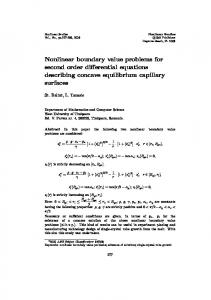
Figure 1: The points (𝑘, 𝑚) (1 ≤ 𝑘, 𝑚 ≤ 10) with integer coordinates such that 𝑘 and 𝑚 satisfy condition (99).

are formulated in terms of eigenvalues of coefficient matrices of linearized systems at zero (at the trivial solution) and at infinity. The proposed approach is applicable to other twopoint boundary conditions such as the Neumann problem and mixed problem.

(98)

Competing Interests

2

Since + + > 𝑘 + 𝑚 > 𝑚 − 𝑘 , one has that 𝜆 1 > 0 and 𝜆 2 < 0. Obviously 𝜆 1 ∉ 𝜎𝐷 = {−(𝑗𝜋)2 : 𝑗 ∈ N}. Note that 𝜆 2 ∉ 𝜎𝐷 also since 𝜆 2 is an algebraic number (𝜆 2 is the root of the characteristic polynomial 𝑝(𝜆) with rational coefficients), but the spectrum 𝜎𝐷 consists of the transcendental numbers (the product −(𝑗𝜋)2 of the algebraic number −𝑗2 with the transcendental number 𝜋2 is transcendental number). Theorem 8 is applicable, taking into account Proposition 3 and Theorem 4, if ind (0, 𝜙) = sgn sin √|𝜆 2 | = −1. Hence, Theorem 8 guarantees the existence of a nontrivial solution to boundary value problem (94) and (95) for all nonzero integers 𝑘 and 𝑚 such that

sin

5

3

Obviously conditions (A1) and (A2) are fulfilled. Due to the boundedness of arctan function, the vector field f is asymptotically linear and f 󸀠 (∞) = 𝑂2 , and hence condition (A3) is fulfilled also. Matrix f 󸀠 (∞) has the only eigenvalue 𝜇 = 0 ∉ 𝜎𝐷, and hence matrix f 󸀠 (∞) does not have negative eigenvalues with odd algebraic multiplicities. It follows from Proposition 6 and Theorem 7 that ind (∞, 𝜙) = 1. −𝑘2 −𝑘2 ) has the characteristic The matrix f 󸀠 (0) = ( −𝑚 2 𝑚2 equation

2 2 2 2 2 𝑚2 − 𝑘2 √(𝑘 + 𝑚 ) + 4𝑘 𝑚 ± . = 2 2

6

4

𝑇

∀x = (𝑥1 , 𝑥2 ) ∈ R2 .

𝑝 (𝜆) = 𝜆2 − (𝑚2 − 𝑘2 ) 𝜆 − 2𝑘2 𝑚2 = 0

m

(99)

The pairs (𝑘, 𝑚) (1 ≤ 𝑘, 𝑚 ≤ 10) with integer coordinates which satisfy condition (99) are depicted in Figure 1.

7. Conclusions For an asymptotically linear system of 𝑛 the second-order ordinary differential equations that are assumed to have the trivial solution to the conditions for existence of nontrivial solutions of the Dirichlet boundary value problem are given. The technique and concepts of the theory of rotation of 𝑛dimensional vector fields are used. The existence conditions

The authors declare that there is no conflict of interests regarding the publication of this paper.

References [1] P. Hartman, Ordinary Differential Equations, John Wiley & Sons, New York, NY, USA, 1964. [2] S. R. Bernfeld and V. Lakshmikantham, An Introduction to Nonlinear Boundary Value Problems, Academic Press, New York, NY, USA, 1974. [3] N. I. Vasilyev and Y. A. Klokov, Foundations of the Theory of Boundary Value Problems for Ordinary Differential Equations, Apgads Zinatne, R¯ıga, Latvia, 1978 (Russian). [4] W. G. Kelley and A. C. Peterson, The Theory of Differential Equations: Classical and Qualitative, Springer, 2010. [5] R. Conti, “Equazioni differenziali ordinarie quasilineari con condizioni lineari,” Annali di Matematica Pura ed Applicata, vol. 57, no. 1, pp. 49–61, 1962. [6] P. Hartman, “On boundary value problems for systems of ordinary, nonlinear, second order differential equations,” Transactions of the American Mathematical Society, vol. 96, no. 3, pp. 493–509, 1960. [7] J. Mawhin, “Boundary value problems for nonlinear secondorder vector differential equations,” Journal of Differential Equations, vol. 16, no. 2, pp. 257–269, 1974. [8] W. T. Reid, “Comparison theorems for non-linear vector differential equations,” Journal of Differential Equations, vol. 5, no. 2, pp. 324–337, 1969.

12 [9] A. Abbondandolo, Morse Theory for Hamiltonian Systems, Chapman & Hall/CRC, 2001. [10] A. Capietto, F. Dalbono, and A. Portaluri, “A multiplicity result for a class of strongly indefinite asymptotically linear second order systems,” Nonlinear Analysis: Theory, Methods & Applications, vol. 72, no. 6, pp. 2874–2890, 2010. [11] A. Capietto, W. Dambrosio, and D. Papini, “Detecting multiplicity for systems of second-order equations: an alternative approach,” Advances in Differential Equations, vol. 10, no. 5, pp. 553–578, 2005. [12] Y. Dong, “Index theory, nontrivial solutions, and asymptotically linear second-order Hamiltonian systems,” Journal of Differential Equations, vol. 214, no. 2, pp. 233–255, 2005. [13] A. Margheri and C. Rebelo, “Multiplicity of solutions of asymptotically linear Dirichlet problems associated to second order equations in R2𝑛+1 ,” Topological Methods in Nonlinear Analysis, vol. 46, no. 2, pp. 1107–1118, 2015. [14] D. O’Regan and R. Precup, Theorems of Leray-Schauder Type and Applications, CRC Press, New York, NY, USA, 2002. [15] R. B. Taher and M. Rachidi, “Linear matrix differential equations of higher-order and applications,” Electronic Journal of Differential Equations, vol. 2008, no. 95, pp. 1–12, 2008. [16] I. Yermachenko and F. Sadyrbaev, “On a problem for a system of two second-order differential equations via the theory of vector fields,” Nonlinear Analysis: Modelling and Control, vol. 20, no. 2, pp. 217–226, 2015. [17] M. A. Krasnosel’ski˘ı, A. I. Perov, A. I. Povolotskiy, and P. P. Zabreiko, Plane Vector Fields, Academic Press, New York, NY, USA, 1966. [18] M. A. Krasnosel’skii, The Operator of Translation Along the Trajectories of Differential Equations, American Mathematical Society, Providence, RI, USA, 1968. [19] V. I. Arnold, Ordinary Differential Equations, Springer, Berlin, Germany, 1992. [20] E. Zehnder, Lectures on Dynamical Systems: Hamiltonian Vector Fields and Symplectic Capacities, European Mathematical Society, Helsinki, Finland, 2010. [21] M. A. Krasnosel’skii and P. P. Zabre˘ıko, Geometrical Methods of Nonlinear Analysis, Springer, Berlin, Germany, 1984. [22] P. P. Zabrejko, “Rotation of vector fields: definition, basic properties, and calculation,” in Topological Nonlinear Analysis II: Degree, Singularity and Variations, M. Matzeu and A. Vignoli, Eds., vol. 27 of Progress in Nonlinear Differential Equations and Their Applications, pp. 445–601, Birkh¨auser, Boston, Mass, USA, 1997. [23] R. A. Horn and C. R. Johnson, Matrix Analysis, Cambridge University Press, London, UK, 1990. [24] F. R. Gantmacher, The Theory of Matrices, AMS Chelsea Publishing, Providence, RI, USA, 1998. [25] V. A. Zorich, Mathematical Analysis I, Springer, Berlin, Germany, 2004.

International Journal of Differential Equations

Advances in

Operations Research Hindawi Publishing Corporation http://www.hindawi.com

Volume 2014

Advances in

Decision Sciences Hindawi Publishing Corporation http://www.hindawi.com

Volume 2014

Journal of

Applied Mathematics

Algebra

Hindawi Publishing Corporation http://www.hindawi.com

Hindawi Publishing Corporation http://www.hindawi.com

Volume 2014

Journal of

Probability and Statistics Volume 2014

The Scientific World Journal Hindawi Publishing Corporation http://www.hindawi.com

Hindawi Publishing Corporation http://www.hindawi.com

Volume 2014

International Journal of

Differential Equations Hindawi Publishing Corporation http://www.hindawi.com

Volume 2014

Volume 2014

Submit your manuscripts at http://www.hindawi.com International Journal of

Advances in

Combinatorics Hindawi Publishing Corporation http://www.hindawi.com

Mathematical Physics Hindawi Publishing Corporation http://www.hindawi.com

Volume 2014

Journal of

Complex Analysis Hindawi Publishing Corporation http://www.hindawi.com

Volume 2014

International Journal of Mathematics and Mathematical Sciences

Mathematical Problems in Engineering

Journal of

Mathematics Hindawi Publishing Corporation http://www.hindawi.com

Volume 2014

Hindawi Publishing Corporation http://www.hindawi.com

Volume 2014

Volume 2014

Hindawi Publishing Corporation http://www.hindawi.com

Volume 2014

Discrete Mathematics

Journal of

Volume 2014

Hindawi Publishing Corporation http://www.hindawi.com

Discrete Dynamics in Nature and Society

Journal of

Function Spaces Hindawi Publishing Corporation http://www.hindawi.com

Abstract and Applied Analysis

Volume 2014

Hindawi Publishing Corporation http://www.hindawi.com

Volume 2014

Hindawi Publishing Corporation http://www.hindawi.com

Volume 2014

International Journal of

Journal of

Stochastic Analysis

Optimization

Hindawi Publishing Corporation http://www.hindawi.com

Hindawi Publishing Corporation http://www.hindawi.com

Volume 2014

Volume 2014