Category: Evolutionary Programming
Discover Probabilistic Knowledge from Databases Using Evolutionary Computation and Minimum Description Length Principle Wai Lam1 1
Man Leung Wong2
Po Shun Ngan3
Department of Systems Engineering and Engineering Management The Chinese University of Hong Kong Shatin Hong Kong 2
3
Wai Lam Man Leung Wong Kwong Sak Leung Po Shun Ngan
Kwong Sak Leung3
Department of Computing and Decision Sciences Lingnan University Tuen Mun Hong Kong
Department of Computer Science and Engineering The Chinese University of Hong Kong Shatin Hong Kong
Email
[email protected] [email protected] [email protected] [email protected]
Phone Numbers 852-2609-8306 852-2616-8093 852-2609-8408
Abstract We have developed a new approach (MDLEP) to learning Bayesian network structures based on the Minimum Description Length (MDL) principle and Evolutionary Programming (EP). It integrates a MDL metric founded on information theory and several new genetic operators including structure-guided operators, a knowledge-guided operator, a freeze operator, and a defrost operator for the discovery process. In contrast, existing techniques based on genetic algorithms (GA) only adopt classical genetic operators. We conduct a series of experiments to demonstrate the performance of our approach and to compare it with that of the GA approach developed in a recent work. The empirical results illustrate that our approach is superior both in terms of quality of the solutions and computational time for data sets we have tested. In particular, our approach can scale up and discover extremely good networks from large benchmark data sets of 10000 cases. Lastly, our MDLEP approach does not need to impose the restriction of having a complete variable ordering as input.
1
1
Introduction
There are different knowledge representation schemes for encoding knowledge. A useful kind of representation is known as a Bayesian network which is an emerging scheme for handling probabilistic knowledge. Many intelligent systems based on this paradigm have been built to perform reasoning under uncertainty e.g., diagnosis, visual recognition, and forecasting [2, 1]. Constructing a Bayesian network manually requires tedious effort from domain experts and knowledge engineers. Thus it is very beneficial if such networks could be automatically discovered from databases. Recently, researchers have begun to work on methods for this discovery problem [10, 6, 19, 3]. It has been shown that this problem is believed to be computationally intractable [5]. Chow and Liu [4] presented an algorithm for learning tree-structured Bayesian networks. Recently a number of research have been conducted to learn multiple-connected network structures. For instance, Herskovits and Cooper developed a Bayesian metric which can measure the fitness of a network structure to the data based on Bayesian approach [6]. A search algorithm called K2 was proposed to find the most desirable network. Heckerman et. al. [10], and Spirtes et. al. [18] proposed various approaches to learn multiple-connected structures. They also developed different network structure construction algorithms and search mechanisms which do not require the variable ordering assumption. More recently, Larranaga et. al. [16, 17] have done some work on using genetic algorithms for learning Bayesian networks. We develop a new approach (MDLEP) to learning multiple-connected network structures based on the MDL principle and Evolutionary Programming (EP). Specifically, our approach employs a MDL-based Bayesian network learning technique founded on information theory and integrates an optimization process which is based on evolutionary programming. An important characteristic of our approach is that, in addition to ordinary genetic operators, we design structure-guided operators and a knowledge-guided operator which incorporates a MDL learning scheme. Essentially we make use of the network structure discovery knowledge for developing the genetic operators. Moreover, a freeze and a defrost operators have been developed to protect good substructures of networks from being modified. In contrast, previous work based on genetic algorithms (GA) do not consider such knowledge in the operators. For instance, Larranaga et. al. [16] used a chromosome to represent a particular variable ordering. The purpose of the genetic operators is to evolve different variable orderings. For each new variable ordering formed by the operators, it is then passed to K2, an existing Bayesian network search algorithm proposed in [6], to obtain a network. In another recent work done by Larranaga et. al. [17], they adopted a classical GA approach and used a chromosome to represent a particular network. Thus the purpose of the genetic operators is to evolve different networks. For each network formed by the operators, it is evaluated using an existing metric mentioned in [6] to measure its merits. However, only simple and standard genetic operators are used. Lastly, our approach does not need to impose the restriction of having a complete variable ordering as input. We conduct a series of experiments to demonstrate the performance of our MDLEP approach and to compare it with that of the classical GA approach described in [17]. The empirical results illustrate that our approach is superior both in terms of quality of the solutions and computational time for data sets we have tested. In particular, our approach can scale up and discover extremely good networks from large benchmark data sets of 10000 cases.
2
Problem Definition
A Bayesian network is composed of a network structure and a set of parameters associated with the structure. In general, the structure consists of nodes which are connected by directed edges and form a directed acyclic graph. Each node represents a domain variable that can take on a finite set of values. Each edge represents a dependency between two nodes. A characteristic of such dependency is that it can be uncertain and is parameterized probabilistically. Formally, let N = {N1 , . . . , Nn } be the set of nodes representing the variables in a domain. Each Ni can instantiate from a finite set of values. In a Bayesian network concerned with N , there is a parent set ΠNi for each node Ni . If Ni has no parent in the network structure, ΠNi is an empty set. This structure captures the fact that the instantiation of node Ni depends on the instantiations of the nodes in ΠNi . Since the dependency can be uncertain, there is a set of conditional probability parameters associated with each node. For node Ni , the probability parameters are in the form of P (Ni | ΠNi ). Figure 1 shows an example of a Bayesian network structure representing the domain of “blue” baby diagnosis. The aim of learning Bayesian networks is to automatically construct such a network model from a database. The network model includes both of the network structure and the associated conditional probability parameters.
2
ND NF
(hypoxia
(duct flow)
distribution)
NL (lower body O2)
NC
NH
(cardiac mixing)
(hypoxia in O2)
Figure 1: A Bayesian Network Structure in a “Blue” Baby Domain The learning problem can also be viewed as a kind of unsupervised learning where the targets to be learned are Bayesian networks. The input data are a collection of cases in a format similar to a table of records in the relational database model. Each case is a fully-instantiated set of domain variables corresponding to some observed real-world circumstance in the domain of interest. Most solutions to the network learning problem divide the problem into two separate phases. In the first phase, a network structure that best characterizes the input data is determined. Then, in the second phase, the conditional probabilities associated with the nodes in the structure are computed. Since once the network structure is known, the conditional probabilities are fixed and can be easily calculated using standard statistical methods. A common way to tackle this learning problem is to focus on the first phase: learning a network structure.
3
A MDL Metric
We briefly describe an approach to Bayesian network structure learning. It is based on our previous work on this problem [15, 14]. Our algorithm makes use of the Minimum Description Length (MDL) principle as a means for balancing between simplicity and accuracy. Central to this approach is a cost metric for a candidate network structure. The cost metric is a function representing the total description length Dt (B) of a candidate network structure B. Within the framework, a shorter length Dt corresponds to a better network. Ideally we would like to find a network structure which has the lowest Dt . We call such a network an optimal network. In situations where an optimal solution cannot be obtained due to limited computing resources, we wish to find a network with Dt as low as possible. In previous work, we have designed a scheme for evaluating this description length [15]. The total description length Dt of a candidate network structure B can be decomposed into each individual variable. Let ΠNi be the parent set of Ni . With overloading of the notation Dt , it can be expressed as: X Dt (B) = Dt (Ni , ΠNi ) Ni ∈N
The total description length Dt is in fact composed of two components: Dt (Ni , ΠNi ) = Dn (Ni , ΠNi ) + Dd (Ni , ΠNi ) where Dn (Ni , ΠNi ) =
Y
ki log2 (n) + d(si − 1)
sj
j∈ΠNi
Dd (Ni , ΠNi ) =
X
M (Ni , ΠNi ) log2
Ni ,ΠNi
M (ΠNi ) M (Ni , ΠNi )
where there are n variables; for variable Ni , ki is the number of its parents, si is the number of values it can take on, and ΠNi is the set of its parents. sj is the number of values a particular variable in ΠNi can take on. d represents the number of bits required to store a numerical value. The summation in the expression for Dd is taken over all possible instantiations of that variable and its parents. M (.) is the number of cases that match a particular instantiation in the database (Note the log function will be 0 if M (Ni ) = 0). Dn and Dd are called the network description length and the data description length, respectively. Network description length has the property that a network with higher topological complexity has a longer description length. Data description length has the property that a more accurate network structure corresponds to a shorter description length. Note that both Dn and Dd are non-negative. 3
4
The MDLEP Learning Approach
4.1
The Algorithm
Our MDLEP approach applies Evolutionary Programming [7, 8] to learn Bayesian network structures. The learning algorithm starts with an initial population of directed acyclic graphs (DAGs) called parents. Each parent is evaluated by using the MDL metric described above. Next, each parent creates an offspring by performing a series of mutations to the parent. The probabilities of executing 1, 2, 3, 4, 5, or 6 times mutations are 0.2, 0.2, 0.2, 0.2, 0.1, and 0.1 respectively. If mutations generate an invalid offspring that is cyclic, the algorithm deletes the edges of the offspring that invalidate the DAG conditions. The new offspring are then evaluated by using the MDL metric. The next generation of parents are selected from the current generation of parents and offspring. The algorithm performs this selection by requiring each DAG to compete against q randomly chosen DAGs. If the MDL metric of the former is lower than or equal to the chosen opponent in each competition, the former receives one score. The algorithm retains the groups of DAGs with the highest scores as parents of the next generation. The algorithm repeats this process until the terminating condition is satisfied. The algorithm is summarized as follows: 1. Set t to 0. 2. Create an initial population, Pop(t), of PS random DAGs. The initial population size is PS. 3. Each DAG in the population Pop(t) is evaluated using the MDL metric. 4. While t is smaller than the maximum number of generation G • Each DAG in Pop(t) produces one offspring by performing a number of mutation operations. If the offspring has cycles, delete the edges of the offspring that violate the DAG condition. • The DAGs in Pop(t) and all new offspring are stored in the intermediate population Pop’(t). The size of Pop’(t) is 2*PS. • Conduct a number of pairwise competitions over all DAGs in Pop’(t). Let Bi be the DAG being conditioned upon, q opponents are selected randomly from Pop’(t) with equal probability. Let Bij , 1 ≤ j ≤ q, be the randomly selected opponent DAGs. The Bi gets one more score if Dt (Bi ) ≤ Dt (Bij ), 1 ≤ j ≤ q. Thus, the maximum score of a DAG is q. • Select PS DAGs with the highest scores from Pop’(t) and store them in the new population Pop(t+1). • Perform freeze and defrost operations to all DAGs in the new population Pop(t+1). • Increase t by 1. 5. Return the DAG with lowest MDL metric found in any generation of a run as the result of the algorithm. In our experiments, we set the value of q to be 5. The learning algorithm uses a variety of structure-guided mutation operators, a knowledge-guided mutation operator, a freeze operator and a defrost operator to produce new offspring from existing DAGs. Formally, let B be an existing DAG to be mutated, N = {N1 , N2 , . . . , Nn } be the set of nodes representing the variables in a domain, E be the set of edges in B. The operators generate a new offspring by modifying E. These operators are detailed in the following sub-sections.
4.2
Structure-Guided Mutation Operators
Simple Mutation: This operator randomly adds an edge eij from nodes Ni to Nj , where i 6= j, if the edge does not already exist. Otherwise, it deletes the edge from E. Reversion: This operator randomly selects an edge, says eij , from E, and modifies the direction of the edge. In other words, the set of edges, E 0 , of the offspring is: E 0 = (E − {eij }) ∪ {eji } Move: This operator modifies the parent set of a node, says Ni , if ΠNi is not empty. Specifically, it deletes a node Nk where Nk ∈ ΠNi , from the parent set of Ni randomly, and adds a new node Nj to ΠNi if Nj 6∈ (ΠNi ∪ {Ni }). 4
4.3
Knowledge-Guided Mutation
This operator is similar to the simple mutation operator. It removes an existing edge from a Bayesian network structure or adds an edge if there is no edge between the corresponding nodes. The main difference between these two operators is that knowledge-guided mutation considers the MDL metric of all possible edges and determines which edge should be removed or inserted. The MDL metric of an edge from Nj to Ni , where i 6= j, is computed by using Dt (Ni , {Nj }). Before the learning algorithm is executed, the MDL metric of all possible edges is computed and stored. When knowledge-guided mutation operator determines that an existing edge of the parental network structure B should be removed, it retrieves the stored MDL metric of all edges in E and those edges with higher MDL metric will be deleted with higher probabilities. On the other hand, if knowledge-guided mutation operator decides to add an edge to the parental network structure, it gets the stored MDL metric of the edges not in E, and the edges with lower MDL metric will have higher probabilities of being added. Recall that the MDL metric of a network structure B is the sum of the MDL metric Dt (Ni , ΠNi ) of all nodes in the network. The objective of the learning algorithm is to find a network structure with minimal MDL metric. Thus, if we want to delete an existing edge from some node to Ni , it is better to select an edge with higher MDL metric because it is more likely to reduce the MDL metric Dt (Ni , ΠNi ) of node Ni . Similarly, if we want to insert an edge from some node to Ni , it is better to select an edge with lower MDL metric because it is more likely to minimize the increment of the MDL metric of node Ni .
4.4
Freeze and Defrost operators
The purpose of the freeze operator is to prevent mutations to a node of a DAG if a number of mutations have been attempted but no improvement can be obtained. A node Ni will be frozen if the following equation returns T rue: ½ n < ≤ GencO−Gen if Genc − Genl ≥ 10 l F reeze(Ni ) = F alse otherwise where < is a random number between 0.0 and 1.0, On is the number of offspring that have been generated by modifying the parent set of Ni , Genc is the current generation number, and Genl is the generation at which the parent set of Ni is obtained. The defrost operator takes a frozen node Nf of a DAG and allows it to be modified again if the following equation returns T rue: On Def rost(Nf ) = R > Genc − Genl
5
Empirical Results and Evaluation
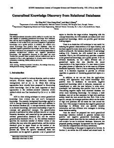
We have conducted a number of experiments to evaluate the performance of our MDLEP approach. We also compare it with a classical GA approach. In each experiment, the learning algorithms attempt to learn a Bayesian network from a data set. The data sets are generated from known Bayesian network structures. To generate the data set, we apply probabilistic logic sampling technique proposed in [12] for a given structure. The learning algorithms take the data set only as input. They do not know the Bayesian networks that generate the data set in any ways during the learning process. After a Bayesian network structure Pn is learned, it is evaluated by two measures. One measure is the structural difference which is defined as: i=1 φi where φi is the sum of the symmetric difference of each parent in the learned network and the known network. Another measure is the total description length Dt . The lower the measure, the better is the network. 10 19
22
21
13
20
31
23
15 34
5
4
11
27
35
32
6
12
36
29
26
3 24
17
18
7
8
9
33
25
16 28
1
37
14
2
30
Figure 2: The ALARM Network Structure
5
The data set PRINTD is derived from a network structure of 26 nodes and 25 arcs. This network structure deals with troubleshooting a printing problem discussed in [11]. 5000 cases was generated. The data set ALARM is derived from a network structure of 36 nodes and 47 arcs as shown in Figure 2. This structure is concerned with a medical domain of potential anesthesia diagnosis in the operating room [2]. We generated 500, 1000, 2000, 3000, 5000, 10000 cases from this structure. The MDL metric of the original network structures for the different data sets are as follows: PRINTD - 106541.62, ALARM 500 cases - 10533.33. ALARM 1000 cases - 18533.45, ALARM 2000 cases - 34287.88, ALARM 3000 cases - 49595.82, ALARM 5000 cases - 81223.41, ALARM 10000 cases - 158497.0.
5.1
Comparison Between MDLEP and GA
We employ our MDLEP learning algorithm to solve the ALARM problem with 500 cases and the PRINTD problem with 5000 cases. The population size PS is 50 and the maximum number of generation is 5000. The probabilities of applying simple mutation, reversion, move, and knowledge-guided mutation are 0.25 each. Ten trials of these experiments were performed. We also implemented a classical genetic algorithm (GA) similar to the work done by [17]. In the GA approach, the MDL metric is used for the objective function. A Bayesian network structure with n nodes is represented by an n × n connectivity matrix C. Each element, cij , is 1 if j is a parent of i. Otherwise, cij is 0. An individual of the population is represented as a string: c11 c21 · · · cn1 c12 c22 · · · cn2 · · · c1n c2n · · · cnn . The one point crossover and mutation operations of classical GA are used [9, 13]. The population size PS is 50 and the maximum number of generation G is 5000. The crossover probability pc is 0.9 and the mutation rate pm is 0.01. Elitist selection is used in the experiments. Ten trials of these experiments are performed. For the ALARM problem with 500 cases, we record the MDL metric of the best Bayesian network of each successive population and calculate the average values of the 10 trials for increasing generations. The MDL metric for our MDLEP learning algorithm and the GA are delineated in Figure 3. We have collected a number of statistics presented in Table 1. • the average of the structural differences of all trials (ASD). • the smallest structural difference of all trials (SSD). • The average of the MDL metric of all trials (AOM). • The smallest MDL metric of all trials (SMM). • The average number of generations (ANG) performed before the best Bayesian network structure is found. • The average number of MDL metric evaluations per Bayesian network structure (AME). If the AME of an algorithm is smaller, the algorithm is relatively faster. • The average size of the parent sets (APS). • The average number of invalid Bayesian network structures produced in each generation (AIB). An algorithm is better if its AIB is lower than that of the other. • The average number of edges deleted in each invalid Bayesian network (AED). If an invalid Bayesian network structure is generated, a number of edges have to be removed to change the invalid network to a valid one. Usually, an invalid network with fewer edges to be deleted is qualitatively better than one with more edges to be removed. Thus, an algorithm is better if its AED is smaller than that of the other algorithm.
MDLEP GA
ASD 24.7 55.9
SSD 20 49
AOM 9764.61 10736.71
SMM 9710.55 10527.04
ANG 4078.5 4384.11
AME 3.88 10.41
APS 1.07 2.13
AIB 9.33 49.34
AED 1.15 5.58
Table 1: Comparison between MDLEP and the GA for the ALARM problem with 500 cases From Figure 3, we can see that MDLEP induces much better Bayesian network structures than the GA. From Table 1, we find that the values of ASD and SSD for MDLEP are 24.7 and 20 respectively. On the other hand, the 6
12000 MDLEP GA
11500
MDL metric
11000 10500 10000 9500 9000 300
900
1500
2100 2700 generation
3300
3900
4500
Figure 3: The MDL metric for the ALARM problem with 500 cases
values of ASD and SSD for the GA are 55.9 and 49 respectively. Consequently, the Bayesian network structures generated by MDLEP are qualitatively better than those obtained by the GA. We find that MDLEP evolves good Bayesian network structures at an average generation of 4078.5. The values of AOM and SMM for MDLEP are 9764.61 and 9710.55 respectively. The values of AOM and SMM for the GA are much higher than those of MDLEP. They are respectively 10736.71 and 10527.04. The GA obtains the solutions at an average generation of 4384. From this information, we can conclude that MDLEP finds much better network structures at earlier generations than the GA. The values of AME, APS, AIB, and AED for MDLEP are smaller than those of the GA, thus MDLEP is better and faster than the GA. For the PRINTD problem with 5000 cases, we record the MDL metric of the best Bayesian network of each successive population and calculate the average values of the 10 trials for increasing generations. The values for MDLEP and the GA are delineated in Figure 4. The structural differences between the best Bayesian network structure found and the original PRINTD network for the two algorithms as well as other statistics can be found in Table 2.
MDLEP GA
107600
MDL metric
107400 107200 107000 106800 106600 300
900
1500
2100 2700 generation
3300
3900
4500
Figure 4: The MDL metric for the PRINTD problem with 5000 cases
MDLEP GA
ASD 0.0 4.7
SSD 0 0
AOM 106541.62 106625.45
SMM 106541.62 106541.62
ANG 468.8 3320.78
AME 3.57 6.30
APS 2.07 2.18
AIB 14.99 38.19
AED 1.22 2.70
Table 2: Comparison between MDLEP and the GA for the PRINTD problem with 5000 cases
We observe from Figure 4 that MDLEP induces better Bayesian network structures than the GA. MDLEP evolves the original PRINTD network structure in all trials. On the other hand, the GA produces the original PRINTD in only one trial. From Table 2, we find that MDLEP evolves good Bayesian network structures at an average generation of 468.8. The values of AOM and SMM for MDLEP are both 106541.62. The values of AOM 7
and SMM for the GA are slightly higher than those of MDLEP. They are respectively 106625.45 and 106541.62. The GA obtains the solutions at an average generation of 3320.78. Thus, MDLEP induces the original PRINTD network structure at much earlier generations than the GA. The values of AME, APS, AIB, and AED for MDLEP are smaller than those of the GA, thus MDLEP is better and faster than the GA.
5.2
Learning the ALARM Network Using MDLEP
In the previous sub-section, we observe that MDLEP is superior to the GA proposed by Larranaga et. al. [17]. Thus, more experiments are done to determine the performance of MDLEP on learning the ALARM network with 500, 1000, 2000, 3000, 5000, and 10000 cases. The parameter values of MDLEP described in the previous sub-section are also used here. Ten trials of each experiment are conducted. A number of statistics are presented in Table 3.
ASD SSD AOM SMM ANG AME APS AIB AED
500 24.7 20 9764.61 9710.55 4078.5 3.88 1.07 9.33 1.15
1000 20.4 15 18025.37 17914.10 4295.6 3.90 1.19 10.84 1.18
2000 11.2 8 33834.54 33745.70 4104.7 3.96 1.34 13.81 1.27
3000 13.1 8 49463.64 49230.10 4304.5 3.94 1.41 14.12 1.29
5000 8.4 6 81043.79 81004.00 3884.3 3.95 1.48 14.78 1.30
10000 9.6 2 158816.10 158420.00 3698.2 4.01 1.54 17.31 1.43
Table 3: Performance of MDLEP for the ALARM problem with 500, 1000, 2000, 3000, 5000 and 10000 cases
From Table 3, we can observe that the values of SMM for all experiments are smaller than the corresponding MDL metric of the original ALARM network given above. In other words, there are Bayesian network structures with smaller MDL metric in the search space and MDLEP can successfully find them in all experiments. The values of ANG show that the best network structures are obtained at generations between 3698 and 4305. The values of AME, APS, AIB, AED for all experiments are within a small interval. However, for a problem with larger number of cases, their values are normally larger than those with smaller number of cases. In other words, the ALARM problem with larger number of cases is harder and takes longer to solve than the one with smaller number of cases. Table 3 indicates that MDLEP can produce network structures that are similar to the original ALARM network. Moreover, if more training cases are available, MDLEP can find better Bayesian networks. Heckerman [10] employed other learning methods to discover the ALARM network with a number of databases of 10000 cases. The ASD of the induced networks is 19.5 and the best one is 8. Our MDLEP approach can learn networks with ASD 9.6 and the best one is 2. Consequently, our approach can learn much better networks.
6
Conclusions
We have presented a novel approach (MDLEP) to learning Bayesian network structures based on the Minimum Description Length (MDL) principle and Evolutionary Programming (EP). Specifically, our approach employs a MDL-based Bayesian network learning technique which is founded on information theory and integrates an optimization process which is based on evolutionary programming. An important characteristic of our approach is that, in addition to ordinary genetic operators, we have designed a freeze operator, a defrost operator, and a knowledge-guided operator which incorporates a MDL learning scheme. Essentially we have made use of the network structure discovery knowledge for developing the genetic operators. We have conducted a series of experiments to demonstrate the performance of our MDLEP approach and to compare the performance of the MDLEP approach with the classical GA approach described in [17]. The empirical results illustrate that our approach is superior both in terms of quality of the solutions and computational time in most data sets we have tested. We plan to further work along a number of directions. One direction is to investigate the technique of using a more specific evolutionary algorithm such as a grammar driven genetic programming to learn the network structures [20].
8
References [1] B. Abramson. ARCO1: An application of belief networks to the oil market. In Proceedings of the Conference on Uncertainty in Artificial Intelligence, pages 1–8, 1991. [2] I. A. Beinlich, H. J. Suermondt, R. M. Chavez, and G. F. Cooper. The ALARM monitoring system: A case study with two probabilistic inference techniques for belief networks. In Proceedings of the 2nd European Conference on Artificial Intelligence in Medicine, pages 247–256, 1989. [3] W. Buntine. Theory refinement on Baysian networks. In Proceedings of the Conference on Uncertainty in Artificial Intelligence, pages 52–60, 1991. [4] C. K. Chow and C. N. Liu. Approximating discrete probability distributions with dependence trees. IEEE Transactions on Information Theory, 14(3):462–467, 1968. [5] G. F. Cooper. The computational complexity of probabilistic inference using Bayesian belief networks. Artificial Intelligence, 42:393–405, 1990. [6] G. F. Cooper and E. Herskovits. A Bayesian method for the induction of probabilistic networks from data. Machine Learning, 9:309–347, 1992. [7] D. B. Fogel. An introduction to simulated evolutionary optimization. IEEE Trans. on Neural Network, 5:3–14, 1994. [8] L. Fogel, A. Owens, and M. Walsh. Artificial Intelligence through Simulated Evolution. New York: John Wiley and Sons, 1966. [9] D. Goldberg. Genetic Algorithms in Search, Optimization, and Machine Learning. Reading MA: Addison-Wesley, 1989. [10] D. Heckerman, D. Geiger, and D. M. Chickering. Learning Bayesian networks: The combination of knowledge and statistical data. Machine Learning, 20(3):197–243, 1995. [11] D. Heckerman and M. Welman. Bayesian networks. Communications of the ACM, 38(8):27–30, 1995. [12] M. Henrion. Propagating uncertainty in Bayesian networks by probabilistic logic sampling. In L. N. Kanal and J. F. Lemmer, editors, Uncertainty in Artificial Intelligence Vol II, pages 149–163. North-Holland, Amsterdam, 1987. [13] J. Holland. Adaptation in Natural and Artificial Systems. Cambridge MA: MIT Press, 1992. [14] W. Lam. Bayesian network refinement via machine learning approach. IEEE Transactions on Pattern Analysis and Machine Intelligence, 1998. To appear. [15] W. Lam and F. Bacchus. Learning Bayesian belief networks - an approach based on the MDL principle. Computational Intelligence, 10(3):269–293, 1994. [16] P. Larranaga, C. Kuijpers, R. Murga, and Y. Yurramendi. Learning Bayesian network structures by searching for the best ordering with genetic algorithms. IEEE Transactions on Systems, Man, and Cybernetics - Part A: Systems and Humans, 26(4):487–493, 1996. [17] P. Larranaga, M. Poza, Y. Yurramendi, R. Murga, and C. Kuijpers. Structure learning of Bayesian network by genetic algorithms: A performance analysis of control parameters. IEEE Transactions on Pattern Analysis and Machine Intelligence, 18(9):912–926, 1996. [18] P. Spirtes, C. Glymour, and R. Scheines. Causation, Prediction, and Search. Springer-Verlag, 1993. [19] P. Spirtes and C. Meek. Learning Bayesian networks with discrete variables from data. In Proceedings of the First International Conference on Knowledge Discovery and Data Mining, pages 294–299, 1995. [20] M.L. Wong and K.S. Leung. Evolutionary program induction directed by logic grammars. Evolutionary Computation, 5(2):143–180, 1997.
9